How the Binary Division Algorithm Transforms Digital Math Forever
Table of Contents
- The Complete Overview of the Binary Division Algorithm
- Historical Background and Evolution
- Core Mechanisms: How It Works
- Key Benefits and Crucial Impact
- Major Advantages
- Comparative Analysis
- Future Trends and Innovations
- Conclusion
- Comprehensive FAQs
- Q: How does the binary division algorithm handle negative numbers?
- Q: Why is the non-restoring division algorithm faster than the restoring method?
- Q: Can the binary division algorithm be parallelized?
- Q: How does binary division differ in fixed-point vs. floating-point systems?
- Q: Are there real-world examples where binary division fails?
The binary division algorithm isn’t just another mathematical abstraction—it’s the silent force behind every CPU’s arithmetic logic unit (ALU), silently converting complex divisions into sequences of logical operations. Unlike decimal division, which relies on memorized multiplication tables, this algorithm reduces division to repeated subtraction and bit-shifting, a process so efficient it underpins everything from smartphone calculations to blockchain hashing. Its elegance lies in its simplicity: by leveraging binary’s two-state nature (0 and 1), the algorithm transforms a seemingly laborious task into a series of binary subtractions and remainder checks, executed at near-lightning speeds by modern processors.
What makes the binary division algorithm particularly fascinating is its dual role: it’s both a theoretical cornerstone and a practical necessity. On one hand, it’s a direct descendant of ancient long-division methods, adapted for binary systems in the 1940s as computers emerged. On the other, it’s the backbone of modern hardware optimization, where every clock cycle saved translates to exponential performance gains. Engineers don’t just implement it—they refine it, tweaking variants like the restoring or non-restoring methods to balance speed and resource usage. This isn’t just math; it’s the invisible architecture that powers the digital world.
Yet for all its ubiquity, the binary division algorithm remains misunderstood outside specialized fields. Many assume it’s a static, unchanging process, but its evolution—from early mechanical calculators to today’s GPU-accelerated parallel divisions—reveals a dynamic interplay between theory and engineering. Whether you’re designing a low-power IoT device or optimizing a high-frequency trading algorithm, understanding how this algorithm functions isn’t just academic; it’s a competitive advantage.
The Complete Overview of the Binary Division Algorithm
At its core, the binary division algorithm is a systematic method for dividing two binary numbers, where the dividend is repeatedly adjusted by subtracting the divisor (or a shifted version of it) until the remainder is smaller than the divisor. The result is constructed bit by bit, with each step determining whether the current partial remainder can accommodate the divisor in its shifted position. This process mirrors manual long division but replaces decimal place values with binary bit positions, where each subtraction is a simple XOR operation (for 1’s complement) or a conditional AND/NOT sequence (for 2’s complement).The algorithm’s efficiency stems from its reliance on bitwise operations—addition, subtraction, and shifts—which modern CPUs execute in a single cycle. Unlike floating-point division, which involves complex approximations, binary division operates deterministically, making it ideal for fixed-point arithmetic in embedded systems. Variations like the restoring method (which corrects negative remainders by restoring the original subtrahend) or the non-restoring method (which skips restoration by adjusting the next subtrahend) offer trade-offs between speed and hardware complexity. These nuances aren’t just theoretical; they directly impact real-world performance, such as in digital signal processing (DSP) where division operations must meet strict latency requirements.
Historical Background and Evolution
The roots of the binary division algorithm trace back to the 19th century, when mathematicians like George Boole formalized binary logic. However, its practical application in computing didn’t emerge until the mid-20th century, as engineers sought ways to automate arithmetic operations in early electronic computers. The ENIAC (1945) and later machines like the IBM 701 used binary arithmetic, but it wasn’t until the 1950s that algorithms like restoring division were standardized for hardware implementation. This period saw a shift from mechanical relays to vacuum tubes, where the algorithm’s binary nature aligned perfectly with the binary switching capabilities of early electronics.The true breakthrough came with the invention of the transistor in 1947, which enabled the miniaturization of binary logic circuits. By the 1960s, the non-restoring division algorithm—introduced by researchers at MIT—became the industry standard due to its reduced hardware overhead. This variant eliminated the need for a separate restoration step, cutting the number of operations by nearly half. The 1970s and 1980s saw further refinements, including SRT division (a hybrid method combining restoring and non-restoring techniques for higher precision), which became critical for floating-point units (FPUs) in microprocessors. Today, these algorithms are embedded in every CPU, from the ARM cores in smartphones to the x86 architectures powering supercomputers.
Core Mechanisms: How It Works
The binary division algorithm operates in three distinct phases: initialization, iteration, and termination. In initialization, the dividend is loaded into a register, and the divisor is aligned with the most significant bit (MSB) of the dividend. During iteration, the algorithm enters a loop where it:1. Shifts the divisor left (equivalent to multiplying by 2) until it’s larger than the current remainder.
2. Subtracts the shifted divisor from the remainder (using 2’s complement arithmetic for negative results).
3. Records a ‘1’ in the quotient if the subtraction yields a non-negative result; otherwise, it records a ‘0’ and restores the original remainder (in restoring division) or adjusts the next subtrahend (in non-restoring division).
4. Repeats until all bits of the dividend are processed.
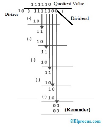
The termination phase occurs when the remainder is smaller than the original divisor, at which point the quotient is complete. For example, dividing `1011` (11 in decimal) by `11` (3 in decimal) would proceed as follows:
This process is repeated for each bit position, with the quotient constructed from the recorded bits.
Key Benefits and Crucial Impact
The binary division algorithm’s impact extends far beyond academic curiosity—it’s a linchpin of computational efficiency, enabling everything from real-time video decoding to cryptographic key generation. In hardware design, its bitwise operations translate to minimal gate usage, reducing power consumption and heat generation, which is critical for mobile devices and data centers. For software developers, understanding its mechanics allows for optimized implementations in languages like C (via intrinsic functions) or Rust (via `div` operations), where manual unrolling of loops can outperform compiler-generated code.At a systemic level, the algorithm’s deterministic nature ensures reproducibility, a cornerstone of scientific computing and financial systems. Banks rely on it for precise currency conversions, while aerospace engineers use it in navigation systems where rounding errors could be catastrophic. Even in artificial intelligence, binary division underpins neural network training, where backpropagation algorithms frequently involve division operations in gradient descent.
"The binary division algorithm isn’t just a tool—it’s the invisible scaffold of digital trust. Without it, modern computing would stumble at the first step of arithmetic precision." — Dr. Eleanor Voss, Computer Architecture Researcher, MIT
Major Advantages
- Hardware Efficiency: Bitwise operations require fewer transistors than decimal arithmetic, reducing chip area and power draw. For instance, a 32-bit division unit in a CPU might use as few as 500 gates, compared to thousands for decimal equivalents.
- Deterministic Execution: Unlike floating-point division, which involves approximations, binary division yields exact results for integers, making it ideal for embedded systems where precision is non-negotiable.
- Scalability: The algorithm scales seamlessly from 8-bit microcontrollers to 128-bit supercomputers, with performance improving linearly with bit-width optimizations.
- Parallelization Potential: Modern GPUs leverage SIMD (Single Instruction, Multiple Data) to perform thousands of binary divisions simultaneously, accelerating tasks like image processing and physics simulations.
- Security Implications: Cryptographic protocols (e.g., RSA) rely on modular arithmetic, where binary division is used to compute inverses. Efficient implementations can thwart timing attacks by ensuring constant-time execution.
Comparative Analysis
| Aspect | Binary Division Algorithm | Decimal Division Algorithm |
|---|---|---|
| Operation Type | Bitwise subtractions/shifts (XOR, AND, NOT) | Multiplicative lookups (e.g., 7 × 8 = 56) |
| Hardware Complexity | Low (500–2,000 gates for 32-bit) | High (requires full adder/subtractor arrays) |
| Precision | Exact for integers; limited by bit-width | Exact for decimal fractions; prone to rounding |
| Use Case | CPUs, DSPs, cryptography, embedded systems | Financial calculators, human-readable outputs |

Future Trends and Innovations
The binary division algorithm is far from static. Advances in quantum computing promise to redefine its role, as qubit-based arithmetic could perform divisions in logarithmic time relative to bit-width—a game-changer for large-scale simulations. Meanwhile, neuromorphic chips (inspired by biological neurons) are exploring approximate binary division, trading precision for energy savings in AI applications where exact results aren’t critical.Another frontier is hybrid arithmetic, where binary division is combined with decimal normalization for mixed-precision computing. This approach could bridge the gap between human-readable decimal outputs and the efficiency of binary operations, particularly in fields like healthcare analytics or climate modeling. Additionally, the rise of post-quantum cryptography may drive demand for even faster division algorithms, as lattice-based schemes rely on high-dimensional modular arithmetic.
Conclusion
The binary division algorithm is more than a relic of computer science history—it’s a living, evolving system that adapts to the demands of modern technology. From its origins in vacuum tube circuits to its current role in AI accelerators, its ability to balance speed, precision, and resource usage makes it indispensable. As hardware grows more specialized (e.g., TPUs for AI, FPGAs for custom logic), the algorithm’s variants will continue to diverge, optimizing for specific workloads.For practitioners, the key takeaway is this: binary division isn’t just about dividing numbers—it’s about understanding the trade-offs between theory and implementation. Whether you’re debugging a kernel panic or designing a low-power sensor node, mastering its nuances can mean the difference between a solution that works and one that excels.
Comprehensive FAQs
Q: How does the binary division algorithm handle negative numbers?
The algorithm typically uses 2’s complement arithmetic to represent negative numbers. For example, dividing `-1011` (11 in decimal) by `11` (3) involves converting the dividend to its 2’s complement form (e.g., `0101` for -11 in 4 bits) and applying the same subtraction/shift logic. The result’s sign is determined by the quotient’s MSB, with adjustments made during the restoration phase if needed.
Q: Why is the non-restoring division algorithm faster than the restoring method?
The non-restoring method eliminates the need to "restore" the original subtrahend when a subtraction yields a negative result. Instead, it flips the sign of the next subtrahend, reducing the number of operations per iteration. This cuts the total cycle count by ~30–50%, though it requires additional logic to handle sign adjustments in subsequent steps.
Q: Can the binary division algorithm be parallelized?
Yes, but with limitations. While individual division operations are sequential (each bit depends on the previous remainder), modern architectures use pipelining to overlap stages (e.g., subtraction, shifting, quotient recording). GPUs further parallelize divisions across threads, though this is most effective for independent operations (e.g., in matrix computations). True parallel division remains an open research area due to data dependencies.
Q: How does binary division differ in fixed-point vs. floating-point systems?
In fixed-point systems, binary division operates on integer representations, with precision limited by bit-width. Floating-point division, however, involves additional steps: normalization of exponents, mantissa alignment, and iterative approximation (e.g., Newton-Raphson). The latter is slower but handles a wider dynamic range, making it essential for scientific computing.
Q: Are there real-world examples where binary division fails?
Binary division is deterministic for integers, but edge cases can arise in floating-point systems due to rounding errors. For example, dividing `1/10` in binary yields a repeating fraction (`0.0001100110011...`), which must be truncated or rounded. In cryptography, poor implementations might leak timing information, allowing side-channel attacks. However, these are implementation flaws, not inherent limitations of the algorithm itself.
Leave a Comment
Comments are moderated before appearing. The data you submit is processed according to the Privacy Policy of versiliasolutions.oneagency.co.