How a Binomial Probability Calculator Transforms Risk Analysis
Table of Contents
- The Complete Overview of Binomial Probability Calculators
- Historical Background and Evolution
- Core Mechanisms: How It Works
- Key Benefits and Crucial Impact
- Major Advantages
- Comparative Analysis
- Future Trends and Innovations
- Conclusion
- Comprehensive FAQs
- Q: Can a binomial probability calculator handle more than two outcomes?
- Q: How does the calculator account for dependent events?
- Q: Why does the calculator sometimes give probabilities greater than 1?
- Q: What’s the difference between "exact" and "cumulative" probability?
- Q: Can I use a binomial calculator for continuous data?
- Q: How do I determine if a binomial approximation is valid?
- Q: Are there free online binomial probability calculators?
- Q: How does sample size affect the calculator’s output?
- Q: Can I use a binomial calculator for hypothesis testing?
- Q: What’s the fastest way to compute binomial probabilities manually?
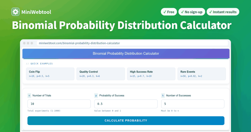
The binomial probability calculator is not just a tool—it’s a precision instrument for quantifying uncertainty in scenarios where outcomes are binary: pass/fail, success/loss, yes/no. Whether you’re a quality control engineer evaluating defect rates in manufacturing or a marketer predicting campaign conversions, the ability to compute exact probabilities for a fixed number of independent trials is transformative. Unlike vague estimates or rule-of-thumb approximations, a binomial probability calculator delivers mathematically rigorous results, bridging the gap between raw data and actionable insights.
What makes this tool uniquely powerful is its adherence to the binomial distribution—a foundational concept in probability theory that models repeated, independent experiments with two possible results. The calculator’s elegance lies in its simplicity: input the number of trials, the probability of success, and the desired number of successes, and it returns the exact probability of that outcome occurring. This precision is critical in fields where even marginal errors can have costly consequences, from pharmaceutical trials to financial forecasting.
Yet, despite its ubiquity in academic and professional settings, the binomial probability calculator remains underleveraged by those outside quantitative disciplines. Many professionals rely on intuition or oversimplified models, unaware that a few keystrokes could reveal probabilities with surgical accuracy. The tool’s versatility—applicable to everything from sports analytics to supply chain logistics—makes it a silent force in decision-making, waiting to be harnessed by those who understand its potential.
The Complete Overview of Binomial Probability Calculators
The binomial probability calculator is a specialized application of combinatorial mathematics, designed to solve problems where events are discrete, binary, and probabilistically independent. At its core, it operationalizes the binomial probability formula:\[ P(X = k) = C(n, k) \times p^k \times (1-p)^{n-k} \]
Here, \( n \) is the number of trials, \( k \) the number of successes, \( p \) the probability of success on a single trial, and \( C(n, k) \) the combination function (n choose k). The calculator automates this computation, eliminating manual errors and accelerating analysis. Its utility spans industries where binary outcomes dominate, such as quality assurance (defective vs. non-defective units), A/B testing (conversion vs. non-conversion), and reliability engineering (system success vs. failure).
Beyond its technical function, the binomial probability calculator serves as a pedagogical tool, demystifying probability theory for practitioners. By visualizing how probabilities shift with changes in \( p \) or \( n \), users gain intuitive grasp of variance and expectation—concepts that underpin statistical inference. For example, a manufacturer testing 100 samples with a 5% defect rate can instantly see the probability of finding 0–5 defects, enabling data-driven adjustments to production processes. This dual role as both a computational aid and an educational resource cements its place in modern analytics.
Historical Background and Evolution
The binomial distribution’s origins trace back to the 17th century, when mathematicians like Blaise Pascal and Pierre de Fermat corresponded on problems of chance, laying the groundwork for combinatorial probability. Their work culminated in the 18th century with Abraham de Moivre’s approximation of the binomial distribution via the normal distribution, a precursor to the central limit theorem. However, it was not until the advent of digital computing in the mid-20th century that the binomial probability calculator became accessible beyond academic circles. Early implementations were clunky, requiring manual input of factorials and powers, but by the 1980s, spreadsheet software like Lotus 1-2-3 integrated binomial functions, democratizing its use.The modern era saw the calculator evolve into user-friendly web and desktop applications, often bundled with statistical software packages like R, Python’s `scipy.stats`, or Excel’s `BINOM.DIST`. These tools refined the interface, adding features like cumulative probability distributions and interactive graphs, while cloud-based calculators further reduced barriers to entry. Today, the binomial probability calculator is as likely to be found in a mobile app as in a research lab, reflecting its transition from a niche academic tool to a mainstream analytical asset.
Core Mechanisms: How It Works
Under the hood, a binomial probability calculator performs three critical operations: combinatorial calculation, probability weighting, and result aggregation. The combination function \( C(n, k) \) determines the number of ways \( k \) successes can occur in \( n \) trials, accounting for all possible sequences (e.g., 2 successes in 5 trials can happen in \( C(5, 2) = 10 \) distinct orders). This is multiplied by \( p^k \), the probability of \( k \) successes, and \( (1-p)^{n-k} \), the probability of \( n-k \) failures. The product yields the exact probability for a specific \( k \). For cumulative probabilities (e.g., "at least 3 successes"), the calculator sums these individual probabilities iteratively.What distinguishes high-quality binomial probability calculators is their handling of edge cases, such as \( p = 0 \) or \( p = 1 \), where the distribution degenerates into deterministic outcomes. Advanced versions also incorporate continuity corrections for large \( n \) and small \( p \), approximating the Poisson distribution when appropriate. The speed of these computations—often instantaneous—stems from optimized algorithms that precompute factorials or use logarithmic transformations to avoid numerical overflow.
Key Benefits and Crucial Impact
The adoption of a binomial probability calculator is not merely a convenience but a strategic advantage. In fields where resources are constrained, the ability to quantify risk with precision allows for better allocation of budgets, time, and effort. For instance, a clinical researcher testing a new drug can use the calculator to determine the minimum sample size needed to achieve statistically significant results, reducing the ethical and financial costs of underpowered trials. Similarly, a logistics manager can predict the likelihood of on-time deliveries given historical failure rates, optimizing inventory levels to minimize stockouts or overstocking.The calculator’s impact extends beyond efficiency to decision transparency. By providing exact probabilities, it replaces guesswork with evidence-based reasoning, a critical feature in regulated industries like healthcare or finance. Where stakeholders demand accountability, the binomial probability calculator delivers quantifiable justification for choices, reducing ambiguity in high-stakes scenarios.
> "Probability is not about predicting the future; it’s about understanding the present with enough clarity to act." > — John Tukey, Statistician
Major Advantages
- Precision Over Estimation: Eliminates approximations by computing exact probabilities, unlike normal approximation methods that introduce error, especially for small \( n \) or extreme \( p \).
- Versatility Across Disciplines: Applicable from manufacturing defect analysis to sports betting, making it a universal tool for binary outcome problems.
- Time Efficiency: Instantaneous results replace hours of manual calculations, accelerating iterative analysis (e.g., sensitivity testing for different \( p \) values).
- Educational Clarity: Interactive calculators with visual outputs (e.g., probability mass functions) help users grasp underlying concepts like variance and skewness.
- Integration with Workflows: Compatible with Excel, Python, R, and cloud platforms, ensuring seamless incorporation into existing analytical pipelines.
Comparative Analysis
| Feature | Binomial Probability Calculator | Normal Approximation | Poisson Approximation |
|---|---|---|---|
| Use Case | Fixed \( n \), binary outcomes (e.g., coin flips, pass/fail tests). | Large \( n \), moderate \( p \) (e.g., \( n > 30 \), \( 0.1 < p < 0.9 \)). | Large \( n \), small \( p \) (e.g., rare events like equipment failures). |
| Accuracy | Exact for all \( n \) and \( p \). | Approximate; errors increase for small \( n \) or \( p \) near 0/1. | Accurate for \( np < 5 \); diverges for larger \( np \). |
| Computational Speed | Instant for typical \( n \) (e.g., \( n < 1000 \)). | Faster for large \( n \) due to simplified formulas. | Fast for sparse events but requires \( np \) checks. |
| Implementation | Standalone tools, Excel, or programming libraries. | Built into most statistical software (e.g., `norm.cdf`). | Specialized for rare-event analysis (e.g., `poisson.pmf`). |

Future Trends and Innovations
The next generation of binomial probability calculators will likely emphasize automation and contextual intelligence. Machine learning models may integrate with calculators to dynamically adjust \( p \) based on real-time data streams, enabling adaptive probability assessments. For example, a retail analytics tool could use historical purchase data to recalibrate the probability of customer churn in real time. Additionally, advancements in natural language processing could allow users to input problems in plain English (e.g., "What’s the chance of 3+ defects in 50 samples if the defect rate is 2%?") and receive instant, visualized results.Another frontier is the fusion of binomial calculators with Bayesian inference, where prior probabilities are updated with new data. This hybrid approach would transform static probability assessments into dynamic, learning systems—ideal for fields like cybersecurity, where threat probabilities evolve continuously. As quantum computing matures, binomial calculations may also benefit from exponential speedups, though practical applications remain years away.
Conclusion
The binomial probability calculator is more than a mathematical utility; it’s a cornerstone of evidence-based decision-making. Its ability to distill complex scenarios into clear probabilities empowers professionals to mitigate risk, optimize resources, and innovate with confidence. While its underlying principles date back centuries, the tool’s modern iterations—now accessible, intuitive, and integrated into broader analytical ecosystems—have redefined its role. As data grows in volume and complexity, the calculator’s precision will become even more critical, ensuring that decisions are not just data-informed but probabilistically rigorous.For those who have yet to leverage it, the binomial probability calculator is a low-effort, high-reward investment. Whether you’re a seasoned statistician or a novice analyst, mastering this tool is the first step toward transforming uncertainty into actionable insight.
Comprehensive FAQs
Q: Can a binomial probability calculator handle more than two outcomes?
A: No. The binomial distribution is strictly for binary outcomes (success/failure). For multinomial outcomes (e.g., three or more categories), use a multinomial probability calculator or a chi-squared test for categorical data.
Q: How does the calculator account for dependent events?
A: It doesn’t. The binomial model assumes independence between trials. If events are dependent (e.g., one trial affects another), use conditional probability or Markov chains instead.
Q: Why does the calculator sometimes give probabilities greater than 1?
A: This never happens in a properly implemented binomial calculator. If you encounter this, check for input errors (e.g., \( p > 1 \) or \( k > n \)) or software bugs. Valid probabilities always sum to 1 across all possible \( k \).
Q: What’s the difference between "exact" and "cumulative" probability?
A: "Exact" probability gives \( P(X = k) \) for a specific \( k \). "Cumulative" probability gives \( P(X \leq k) \) or \( P(X \geq k) \), summing probabilities across a range of \( k \) values. Most calculators offer both options.
Q: Can I use a binomial calculator for continuous data?
A: No. The binomial distribution is discrete. For continuous data (e.g., heights, temperatures), use the normal, exponential, or other continuous distributions. Discretizing continuous data (e.g., rounding) can approximate binomial scenarios but introduces approximation errors.
Q: How do I determine if a binomial approximation is valid?
A: The normal approximation is valid if \( n \times p \geq 5 \) and \( n \times (1-p) \geq 5 \). The Poisson approximation is valid if \( n \) is large and \( p \) is small (typically \( n \geq 20 \) and \( p \leq 0.05 \)). For edge cases, use the exact binomial formula.
Q: Are there free online binomial probability calculators?
A: Yes. Reputable options include:
- Calculator.net’s Binomial Calculator
- Omni Calculator’s Binomial Distribution Calculator
- Excel’s `BINOM.DIST` function (accessible via free Office Online)
Q: How does sample size affect the calculator’s output?
A: Larger \( n \) increases the precision of the binomial distribution, making it more symmetric and approximating a normal distribution (by the Central Limit Theorem). For small \( n \), the distribution is skewed, especially if \( p \) is near 0 or 1.
Q: Can I use a binomial calculator for hypothesis testing?
A: Indirectly, yes. You can compute probabilities for observed outcomes (e.g., "What’s the chance of seeing 8+ successes if \( p = 0.5 \)?"), then compare to a significance threshold (e.g., \( \alpha = 0.05 \)). For formal hypothesis tests, use binomial tests or chi-squared tests in statistical software.
Q: What’s the fastest way to compute binomial probabilities manually?
A: Use the multiplicative formula:
\[ P(X = k) = \frac{n!}{k!(n-k)!} \times p^k \times (1-p)^{n-k} \]
For large \( n \), precompute factorials or use logarithms to simplify calculations. Tools like graphing calculators (e.g., TI-84) also have built-in binomial functions.
Leave a Comment
Comments are moderated before appearing. The data you submit is processed according to the Privacy Policy of versiliasolutions.oneagency.co.