How to Calculate Sampling Distribution: The Definitive Statistical Framework
Table of Contents
- The Complete Overview of Calculating Sampling Distribution
- Historical Background and Evolution
- Core Mechanisms: How It Works
- Key Benefits and Crucial Impact
- Major Advantages
- Comparative Analysis
- Future Trends and Innovations
- Conclusion
- Comprehensive FAQs
- Q: What’s the difference between a sampling distribution and a probability distribution?
- Q: Can I calculate sampling distribution for small samples?
- Q: How does sample size affect the sampling distribution?
- Q: Is bootstrapping always better than theoretical methods?
- Q: What’s the role of the Central Limit Theorem in calculating sampling distribution?
- Q: How do I handle non-normal sampling distributions?
Sampling distributions are the invisible scaffolding of modern statistics, transforming raw data into actionable insights. Without them, confidence intervals would crumble, hypothesis tests would fail, and entire fields—from clinical trials to market research—would lack the rigor to draw conclusions. Yet, despite their ubiquity, the process of calculating sampling distribution remains misunderstood, often reduced to abstract formulas rather than a practical toolkit for decision-making.
The stakes are higher than ever. In an era where data-driven decisions dictate everything from policy formulation to corporate strategy, the ability to determine sampling distribution accurately separates competent analysts from those who stumble into costly errors. Whether you’re a researcher validating a survey’s reliability or a data scientist optimizing machine learning models, grasping how to derive sampling distribution is non-negotiable. It’s not just about numbers—it’s about understanding the behavior of those numbers under repeated sampling.
The confusion begins with terminology. Many conflate sampling distributions with population parameters or confuse them with probability distributions. Others treat the process as a black box, applying formulas without intuition. But calculating sampling distribution is a systematic exercise in probability theory, rooted in the Central Limit Theorem (CLT) and the law of large numbers. It’s where theory meets application, where abstract concepts like bias and variance become tangible levers for improving data quality.
The Complete Overview of Calculating Sampling Distribution
At its core, calculating sampling distribution refers to the process of deriving the probability distribution of a statistic (e.g., mean, proportion) obtained from a large number of random samples drawn from a population. This isn’t just academic—it’s the foundation of inferential statistics, enabling researchers to estimate population characteristics with measurable uncertainty. For example, when polling voters, statisticians don’t rely on a single sample’s mean; they calculate sampling distribution to quantify how much that mean might vary if the survey were repeated, ensuring results are statistically significant rather than just lucky.The method hinges on three pillars: random sampling, sample size, and statistical properties (mean, variance). Random sampling ensures each subset of the population has an equal chance of selection, while sample size dictates the precision of the distribution. The statistical properties—particularly the mean of the sampling distribution (which equals the population mean) and its standard error (a function of sample size)—are what allow analysts to determine sampling distribution with confidence. Without these, the entire framework collapses into guesswork.
Historical Background and Evolution
The concept of sampling distributions emerged in the early 20th century as statisticians sought to bridge the gap between theoretical probability and real-world data. Karl Pearson’s work on correlation in the 1890s laid early groundwork, but it was Ronald Fisher and Jerzy Neyman who formalized the principles in the 1920s–30s. Fisher’s introduction of the t-distribution for small samples and Neyman’s development of confidence intervals provided the tools to calculate sampling distribution for means and proportions, revolutionizing fields like agriculture and medicine.The Central Limit Theorem (CLT), first articulated by Laplace in the early 1800s but refined by later statisticians, became the cornerstone of sampling theory. The CLT states that, regardless of the population’s shape, the sampling distribution of the mean will approximate a normal distribution as sample size grows—a discovery that democratized statistical inference. By the mid-20th century, computers made it feasible to simulate sampling distributions empirically, shifting the focus from theoretical derivation to practical application. Today, determining sampling distribution is as likely to involve Monte Carlo simulations as it is classical formulas.
Core Mechanisms: How It Works
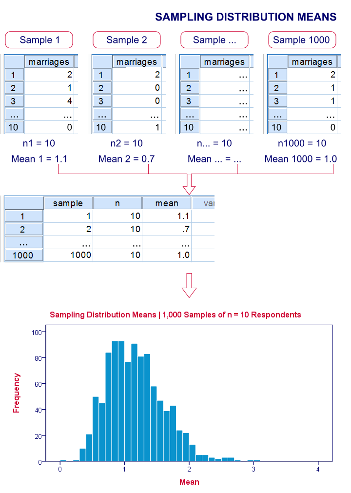
To calculate sampling distribution for a statistic like the sample mean, follow these steps:1. Define the Population Parameter: Identify the target statistic (e.g., population mean μ).
2. Specify Sample Size (n): Larger samples yield tighter distributions (lower standard error).
3. Draw Repeated Samples: Use random sampling to generate multiple subsets of size n.
4. Compute the Statistic: For each sample, calculate the mean (or other statistic of interest).
5. Plot the Results: The distribution of these means is the sampling distribution.
The key insight is that the sampling distribution’s standard error (SE) is given by:
\[ SE = \frac{\sigma}{\sqrt{n}} \]
where σ is the population standard deviation. This formula explains why increasing sample size reduces variability—a principle exploited in quality control, clinical trials, and A/B testing.
For proportions, the process mirrors this but uses the binomial distribution’s properties. The sampling distribution of a sample proportion p̂ has:
Key Benefits and Crucial Impact
The ability to calculate sampling distribution is the difference between anecdotal evidence and empirical proof. It allows researchers to quantify uncertainty, ensuring that conclusions aren’t overstated. In drug trials, for instance, determining sampling distribution for treatment effects ensures patient safety by ruling out false positives. In economics, it validates policy impacts by accounting for sampling variability. Even in everyday contexts—like estimating election outcomes—the same principles underpin exit poll projections.Without sampling distributions, confidence intervals would lack rigor, p-values would be meaningless, and entire industries would operate on shaky foundations. The discipline forces analysts to confront a fundamental question: How much can I trust this result? The answer lies in the sampling distribution’s shape, spread, and central tendency.
"Statistics is the grammar of science. Sampling distributions are its syntax—the rules that turn data into coherent arguments." — George E. P. Box, Statistician
Major Advantages
- Precision in Estimation: By calculating sampling distribution, analysts can construct confidence intervals that reflect true uncertainty, not just point estimates.
- Hypothesis Testing: The sampling distribution underpins t-tests, z-tests, and chi-square tests, enabling rigorous comparisons between groups.
- Resource Optimization: Knowing the standard error helps determine optimal sample sizes, balancing cost and accuracy.
- Robustness to Non-Normality: The CLT ensures determining sampling distribution works even for skewed populations, given sufficient sample size.
- Reproducibility: Sampling distributions provide a framework to validate results across different studies or datasets.
Comparative Analysis
| Method | Use Case |
|---|---|
| Analytical (Theoretical)Using CLT/formulas to derive sampling distribution. | Ideal for large samples where population parameters (μ, σ) are known. |
| Empirical (Bootstrapping)Resampling from observed data to estimate sampling distribution. | Useful when population parameters are unknown or data is limited. |
| Simulation (Monte Carlo)Generating synthetic samples to model sampling distribution. | Best for complex scenarios (e.g., stratified sampling, non-normal distributions). |
| Bayesian ApproachesCombining prior distributions with likelihood to infer sampling distribution. | Preferred when incorporating expert knowledge or small datasets. |

Future Trends and Innovations
The future of calculating sampling distribution lies in integration with machine learning and big data. Traditional methods assumed i.i.d. (independent and identically distributed) samples, but modern datasets often violate this (e.g., time-series, hierarchical structures). Innovations like Bayesian hierarchical models and deep learning-based resampling are expanding how we determine sampling distribution in non-standard contexts.Another frontier is causal inference, where sampling distributions help estimate treatment effects while accounting for confounding variables. Tools like doubly robust estimation and synthetic controls rely on sophisticated sampling distribution frameworks to deliver unbiased results. As data grows messier, the ability to calculate sampling distribution accurately will remain the litmus test for statistical validity.
Conclusion
Calculating sampling distribution is not a one-time calculation but a continuous process of refinement. It demands a blend of theoretical rigor and practical adaptability—whether you’re applying the CLT to a survey or bootstrapping a complex dataset. The discipline ensures that every inference, from academic research to corporate analytics, is grounded in probability rather than intuition.For practitioners, the takeaway is clear: Master the mechanics, but never lose sight of the goal. The sampling distribution isn’t just a mathematical curiosity; it’s the bridge between data and decision-making. Ignore it at your peril.
Comprehensive FAQs
Q: What’s the difference between a sampling distribution and a probability distribution?
A: A probability distribution describes the likelihood of all possible outcomes in a population (e.g., normal distribution of heights). A sampling distribution, however, shows how a statistic (like the mean) behaves across repeated samples. For example, the sampling distribution of the mean is centered on the population mean but with its own variance (standard error).
Q: Can I calculate sampling distribution for small samples?
A: Yes, but the Central Limit Theorem (CLT) requires larger samples (n ≥ 30) for normality. For small samples, use the t-distribution (if population σ is unknown) or bootstrapping to empirically estimate the sampling distribution. The t-distribution accounts for higher variability in small samples.
Q: How does sample size affect the sampling distribution?
A: Increasing sample size (n) reduces the standard error (SE = σ/√n), making the sampling distribution narrower and more precise. For example, doubling n from 100 to 200 halves the SE, tightening confidence intervals. This is why large samples are critical for detecting small effects.
Q: Is bootstrapping always better than theoretical methods?
A: Not necessarily. Bootstrapping is powerful for complex distributions or unknown parameters but can be computationally intensive and may introduce bias if the resampling isn’t representative. Theoretical methods (e.g., CLT) are faster and more interpretable when assumptions hold. Choose based on data quality and computational resources.
Q: What’s the role of the Central Limit Theorem in calculating sampling distribution?
A: The CLT guarantees that, regardless of the population’s shape, the sampling distribution of the mean will approximate a normal distribution as n increases. This allows analysts to use z-tests or t-tests even for non-normal data, provided n is sufficiently large (typically n > 30). Without the CLT, many inferential tools would be unusable.
Q: How do I handle non-normal sampling distributions?
A: If the sampling distribution is skewed or heavy-tailed, consider:
Leave a Comment
Comments are moderated before appearing. The data you submit is processed according to the Privacy Policy of versiliasolutions.oneagency.co.