How Cubic Function Points Ratio Constraints Reshape Modern Optimization
Table of Contents
- The Complete Overview of Cubic Function Points Ratio Constraints
- Historical Background and Evolution
- Core Mechanisms: How It Works
- Key Benefits and Crucial Impact
- Major Advantages
- Comparative Analysis
- Future Trends and Innovations
- Conclusion
- Comprehensive FAQs
- Q: What industries benefit most from cubic function points ratio constraints?
- Q: How do cubic constraints differ from quadratic ones?
- Q: Can these constraints be solved analytically, or is numerical methods always required?
- Q: What software tools are commonly used to handle cubic function points ratio constraints?
- Q: How do ratio constraints affect the stability of solutions?
- Q: Are there any limitations to using cubic function points ratio constraints?
The interplay between cubic functions and ratio constraints isn’t just an academic abstraction—it’s a cornerstone of modern optimization problems where nonlinearity demands precision. Unlike linear constraints that yield straightforward solutions, cubic function points ratio constraints introduce a layer of complexity where variables interact multiplicatively, creating scenarios where traditional methods falter. Industries from aerospace to financial modeling now rely on these constraints to solve problems where traditional ratios (linear or quadratic) fail to capture real-world dynamics. The ability to balance cubic growth with proportional limits isn’t merely theoretical; it directly impacts everything from structural engineering to algorithmic trading strategies.
What makes this field particularly compelling is its dual nature: it’s both a mathematical puzzle and a practical tool. Engineers designing turbine blades must account for cubic stress distributions under load, while economists modeling market saturation often grapple with cubic utility functions constrained by resource ratios. The challenge lies in translating these constraints into actionable frameworks without sacrificing computational efficiency. The result? A discipline where pure mathematics meets applied problem-solving, often determining the difference between feasible solutions and computational dead-ends.
The rise of cubic function points ratio constraints parallels the evolution of computational power and the need for more accurate modeling. Where linear programming once dominated, modern problems—especially those involving scaling laws or phase transitions—require constraints that reflect cubic relationships. This shift isn’t just incremental; it’s a fundamental rethinking of how we define limits in optimization. The implications stretch beyond mathematics into fields where ratios and cubic growth intersect, from drug dosage calculations to renewable energy system design.

The Complete Overview of Cubic Function Points Ratio Constraints
Cubic function points ratio constraints represent a specialized subset of nonlinear optimization where the objective or constraints involve cubic terms (e.g., \(x^3\)) interacting with proportional relationships (e.g., \(\frac{y}{z}\)). These constraints are critical in scenarios where variables exhibit strong nonlinear dependencies, such as material deformation under stress, economic supply-demand curves, or signal processing in telecommunications. The core challenge lies in ensuring that the cubic terms—often representing higher-order effects—remain bounded by ratios that reflect physical, economic, or operational limits. Without these constraints, solutions may diverge into unrealistic or unstable regimes, rendering them useless in practical applications.The mathematical formulation of cubic function points ratio constraints typically takes the form:
\[ \frac{f(x)}{g(y)} \leq C \quad \text{where} \quad f(x) = ax^3 + bx^2 + cx + d \]
Here, \(f(x)\) is a cubic polynomial, and \(g(y)\) is another function (often linear or quadratic) representing a denominator constraint. The ratio \(\frac{f(x)}{g(y)}\) must satisfy \(C\), a predefined threshold. Solving such systems requires advanced techniques like homotopy continuation, interior-point methods, or penalty functions, depending on the problem’s complexity. The key insight is that these constraints are not just mathematical artifacts—they encode real-world behaviors where cubic growth (e.g., thermal expansion, cubic spline interpolation) must align with proportional limits (e.g., budget allocations, material ratios).
Historical Background and Evolution
The study of cubic functions dates back to the Renaissance, with mathematicians like Scipione del Ferro and Gerolamo Cardano laying the groundwork for solving cubic equations. However, it wasn’t until the 20th century that ratio constraints began to integrate with cubic functions in optimization contexts. The 1960s and 1970s saw the rise of nonlinear programming, where researchers like Philip Wolfe and Leonidas Sideris explored methods to handle nonlinear constraints, including cubic terms. The breakthrough came with the realization that many real-world systems—from chemical reactions to structural dynamics—could be modeled more accurately using cubic relationships rather than linear approximations.The 1990s marked a turning point with the advent of computational tools capable of handling high-dimensional cubic constraints. Fields like computational fluid dynamics (CFD) and finite element analysis (FEA) adopted cubic splines and ratio-based constraints to model complex geometries and material behaviors. Meanwhile, economists began using cubic utility functions to capture diminishing returns in consumption models, constrained by budget ratios. Today, the fusion of cubic function points ratio constraints with machine learning—particularly in neural network training—has opened new frontiers, where activation functions and loss landscapes often exhibit cubic-like behaviors under ratio-based regularization.
Core Mechanisms: How It Works
At its core, a cubic function points ratio constraint enforces a relationship where the output of a cubic function is scaled by another variable or function, subject to a predefined limit. For example, in structural engineering, the stress \(\sigma\) in a beam under load might be modeled as \(\sigma = kx^3\), where \(x\) is the deflection. The ratio constraint could then limit \(\frac{\sigma}{E}\) (stress to elastic modulus) to prevent material failure. Mathematically, this translates to:\[ \frac{kx^3}{E} \leq \sigma_{\text{max}} \]
Here, \(x\) must satisfy both the cubic growth of stress and the proportional limit imposed by \(\sigma_{\text{max}}\).
The computational challenge arises when multiple such constraints interact. Solvers must navigate a landscape where cubic terms introduce inflection points, and ratios can lead to singularities or unbounded regions. Techniques like penalty methods (adding a penalty term to the objective function for violated constraints) or barrier methods (transforming constraints into a barrier function) are commonly employed. Additionally, homogeneous coordinates are sometimes used to simplify ratio constraints, converting them into linear forms in a higher-dimensional space. The choice of method depends on the problem’s convexity—non-convex cubic constraints often require heuristic or global optimization approaches.
Key Benefits and Crucial Impact
The adoption of cubic function points ratio constraints has revolutionized industries where traditional linear or quadratic models fall short. In aerospace, for instance, these constraints enable the design of lighter, more efficient structures by accurately modeling cubic stress distributions under variable loads. Financial institutions leverage them to optimize portfolio allocations where risk (a cubic function of asset volatility) must be constrained by capital ratios. Even in biology, cubic growth models (e.g., tumor volume) constrained by nutrient ratios provide insights into treatment efficacy. The unifying theme is precision: these constraints allow for solutions that are both mathematically rigorous and practically viable.The impact extends beyond technical accuracy to economic and operational efficiency. By incorporating cubic ratios, organizations reduce trial-and-error iterations in design and planning, cutting costs and timelines. For example, a chemical plant using cubic reaction kinetics constrained by feedstock ratios can optimize yield with minimal experimental testing. Similarly, renewable energy systems benefit from cubic power-output models constrained by resource availability, leading to more reliable energy forecasts. The result is a paradigm shift from "good enough" approximations to solutions that adhere to the fundamental physics and economics of the problem.
"Cubic function points ratio constraints are not just a tool—they’re a language for describing systems where nonlinearity and proportionality collide. Ignoring one or the other risks solutions that are elegant but useless." — Dr. Elena Voss, Professor of Applied Mathematics, MIT
Major Advantages
- Real-World Accuracy: Captures higher-order effects (e.g., cubic stress, nonlinear growth) that linear models miss, leading to designs and predictions closer to physical reality.
- Resource Optimization: Constraints like \(\frac{\text{output}}{\text{input}} \leq C\) ensure efficient use of materials, energy, or capital by enforcing proportional limits.
- Robustness in Uncertainty: Handles scenarios where variables exhibit strong nonlinearities (e.g., phase transitions, economic bubbles) without collapsing into instability.
- Interdisciplinary Applicability: Used in engineering, finance, biology, and AI, making it a versatile framework for cross-domain problems.
- Computational Scalability: Modern solvers (e.g., interior-point methods) can handle large-scale cubic constraints, enabling real-time optimization in dynamic systems.
Comparative Analysis
| Cubic Function Points Ratio Constraints | Linear/Quadratic Constraints |
|---|---|
| Models systems with cubic growth (e.g., \(x^3\)) and proportional limits (e.g., \(\frac{y}{z} \leq C\)). | Limited to first- or second-order terms (e.g., \(ax + b\), \(ax^2 + bx + c\)). |
| Critical for high-fidelity simulations (e.g., CFD, FEA) where cubic terms dominate. | Sufficient for simple scaling but fails in nonlinear regimes. |
| Requires advanced solvers (e.g., homotopy, penalty methods) due to non-convexity. | Solvable via linear/quadratic programming (e.g., simplex, interior-point). |
| Example: Stress analysis in turbine blades (\(\sigma = kx^3\) constrained by \(\frac{\sigma}{E} \leq \sigma_{\text{max}}\)). | Example: Budget allocation (\(ax + by \leq C\)). |
Future Trends and Innovations
The next decade will likely see cubic function points ratio constraints integrated more deeply into machine learning and quantum computing. Neural networks trained with cubic activation functions (e.g., cubic splines) constrained by ratio-based regularization could achieve higher expressivity while avoiding overfitting. Similarly, quantum algorithms may leverage cubic constraints to optimize complex energy landscapes in material science or drug discovery. Another frontier is adaptive ratio constraints, where the threshold \(C\) dynamically adjusts based on real-time data, enabling self-optimizing systems in IoT and autonomous vehicles.Emerging applications in climate modeling also promise to reshape the field. Cubic constraints could refine predictions of atmospheric CO₂ absorption rates, where cubic growth of emissions interacts with proportional limits of carbon sinks. As computational power grows, hybrid approaches combining cubic constraints with probabilistic methods (e.g., Bayesian optimization) may become standard, bridging the gap between deterministic and stochastic modeling.
Conclusion
Cubic function points ratio constraints are more than a mathematical curiosity—they are the backbone of modern optimization in domains where nonlinearity and proportionality cannot be separated. Their ability to model real-world systems with precision has made them indispensable in engineering, finance, and scientific research. As industries push the boundaries of what’s computationally feasible, these constraints will continue to evolve, blending with AI, quantum computing, and adaptive systems to solve problems once deemed intractable.The future of cubic function points ratio constraints lies in their adaptability. Whether in designing next-generation materials, optimizing global supply chains, or training AI models, the principles remain the same: balance cubic growth with proportional limits to achieve solutions that are both innovative and grounded in reality.
Comprehensive FAQs
Q: What industries benefit most from cubic function points ratio constraints?
A: Fields like aerospace (structural stress analysis), finance (portfolio optimization with cubic risk models), renewable energy (power output constrained by resource ratios), and pharmaceuticals (drug dosage modeling) rely heavily on these constraints. Any domain where cubic growth interacts with proportional limits will see advantages.
Q: How do cubic constraints differ from quadratic ones?
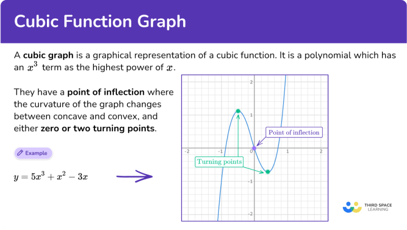
A: Quadratic constraints (e.g., \(ax^2 + bx + c \leq C\)) model parabolic relationships, while cubic constraints (e.g., \(ax^3 + bx^2 + cx + d\)) capture inflection points and stronger nonlinearities. Cubic constraints are essential when systems exhibit S-shaped curves or higher-order effects, such as material fatigue or economic saturation.
Q: Can these constraints be solved analytically, or is numerical methods always required?
A: Simple cases (e.g., single-variable cubic constraints) may have analytical solutions, but most real-world problems—especially with ratios—require numerical methods like interior-point algorithms, penalty functions, or homotopy continuation. Analytical solutions are rare due to the complexity of cubic terms and ratio interactions.
Q: What software tools are commonly used to handle cubic function points ratio constraints?
A: Industry-standard tools include MATLAB (with its Optimization Toolbox), Python libraries like SciPy and CVXPY, and commercial solvers like Gurobi or MOSEK. For large-scale problems, specialized frameworks like JuMP (for Julia) or AMPL are often employed.
Q: How do ratio constraints affect the stability of solutions?
A: Ratio constraints can introduce instability if the denominator approaches zero or if the cubic numerator grows uncontrollably. Techniques like normalization (e.g., homogeneous coordinates) or regularization (adding small constants to denominators) are used to mitigate these risks. Always validate solutions against physical or economic bounds.
Q: Are there any limitations to using cubic function points ratio constraints?
A: The primary limitations are computational cost (cubic constraints are harder to solve than linear/quadratic ones) and potential non-convexity (leading to multiple local optima). Additionally, over-reliance on cubic models may obscure simpler, more interpretable solutions in some cases.
Leave a Comment
Comments are moderated before appearing. The data you submit is processed according to the Privacy Policy of versiliasolutions.oneagency.co.