How the Diagonalization Matrix Calculator Transforms Linear Algebra Workflows
Table of Contents
- The Complete Overview of Diagonalization Matrix Calculators
- Historical Background and Evolution
- Core Mechanisms: How It Works
- Key Benefits and Crucial Impact
- Major Advantages
- Comparative Analysis
- Future Trends and Innovations
- Conclusion
- Comprehensive FAQs
- Q: Can a diagonalization matrix calculator handle non-diagonalizable matrices?
- Q: How do I choose between an online calculator and a library-based tool?
- Q: What’s the most numerically stable method for diagonalization?
- Q: Why might my calculator return complex eigenvalues for a real matrix?
- Q: Are there calculators optimized for specific hardware (e.g., GPUs)?h3> A: Yes. Libraries like CuBLAS (NVIDIA’s GPU-accelerated BLAS) and PyTorch’s linear algebra functions leverage GPU parallelism to diagonalize large matrices orders of magnitude faster than CPU-only tools. For example, diagonalizing a 10,000×10,000 matrix on a GPU can reduce runtime from hours to minutes. Frameworks like RAPIDS cuDF also provide GPU-optimized diagonalization for dataframes. Q: How can I verify the accuracy of a diagonalization result?
The diagonalization of matrices isn’t just an abstract concept—it’s the backbone of modern data science, quantum computing, and machine learning. When engineers at NASA’s Jet Propulsion Laboratory need to stabilize satellite trajectories or researchers at MIT’s AI lab fine-tune neural network weights, they rely on tools that can efficiently compute diagonalizable matrices. These tools, often referred to as diagonalization matrix calculators, bridge theoretical mathematics with practical computational power. Without them, tasks like principal component analysis (PCA) or solving coupled differential equations would grind to a halt, forcing experts to resort to tedious manual calculations or brute-force numerical methods.
Yet for all their utility, these calculators remain shrouded in complexity for many practitioners. The average user might understand the concept of diagonalization—transforming a matrix into a simpler diagonal form—but few grasp how the underlying algorithms handle edge cases like defective matrices or non-diagonalizable systems. The gap between theory and implementation is where the real value lies, and where a diagonalization matrix calculator becomes indispensable. It doesn’t just perform calculations; it democratizes access to advanced linear algebra, allowing researchers, students, and engineers to focus on interpretation rather than computation.
The evolution of these tools mirrors the broader trajectory of computational mathematics. What began as pen-and-paper exercises in the 19th century has now been distilled into high-performance libraries like NumPy, MATLAB’s `eig()` function, or specialized online calculators. Today’s diagonalization matrix calculators don’t just compute eigenvalues and eigenvectors—they optimize for speed, handle large-scale sparse matrices, and even provide visualizations of spectral properties. But beneath the polished interfaces lies a rigorous mathematical framework, one that demands precision in both algorithmic design and numerical stability.
The Complete Overview of Diagonalization Matrix Calculators
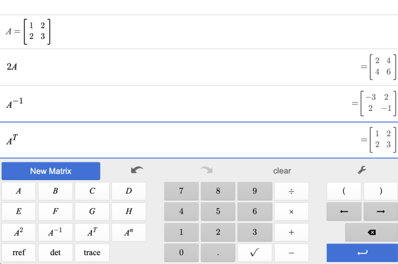
At its core, a diagonalization matrix calculator is a computational tool designed to decompose a square matrix into its diagonalizable form, if possible. This process involves finding a matrix \( P \) (whose columns are eigenvectors) and a diagonal matrix \( D \) (whose entries are eigenvalues) such that \( A = PDP^{-1} \). The calculator automates this decomposition, handling everything from input validation to numerical approximations when exact solutions aren’t feasible. For matrices that aren’t diagonalizable—those with deficient eigenvector sets—the tool may instead compute a Jordan canonical form or apply Schur decomposition as a fallback.The practical applications of these calculators extend far beyond academic exercises. In quantum mechanics, diagonalization reveals energy levels of particles; in economics, it simplifies input-output models; and in computer graphics, it accelerates transformations. Even in everyday technology, algorithms for image compression (like JPEG) rely on diagonalizable matrices to reduce dimensionality. The calculator’s role isn’t just about solving equations—it’s about enabling discoveries that would otherwise require years of manual labor.
Historical Background and Evolution
The mathematical foundations of diagonalization trace back to the 18th century, when Leonhard Euler and Joseph-Louis Lagrange explored the properties of quadratic forms. However, it was the 19th-century work of Cauchy, Hamilton, and Sylvester that formalized the concept of eigenvalues and eigenvectors. By the early 20th century, mathematicians like David Hilbert and Hermann Weyl had connected diagonalization to spectral theory, laying the groundwork for functional analysis. The real turning point came with the advent of digital computers in the mid-1900s, when numerical algorithms—such as the QR algorithm for eigenvalue computation—were developed to handle large matrices efficiently.Today’s diagonalization matrix calculators are the culmination of over two centuries of theoretical and applied research. Early implementations in the 1960s and 70s were limited by hardware constraints, but advancements in floating-point arithmetic and parallel processing have since transformed these tools into high-precision engines. Modern calculators leverage libraries like LAPACK (Linear Algebra Package) and BLAS (Basic Linear Algebra Subprograms), which are optimized for performance across different hardware architectures, from CPUs to GPUs. Even open-source platforms like Python’s SciPy now offer built-in functions like `scipy.linalg.eigh` that abstract away much of the complexity, making diagonalization accessible to non-experts.
Core Mechanisms: How It Works
Under the hood, a diagonalization matrix calculator employs a combination of direct and iterative methods to decompose a matrix. For small, dense matrices, direct methods like the QR algorithm or divide-and-conquer approaches (e.g., the Francis QR algorithm) are preferred. These methods iteratively transform the matrix into upper triangular form, from which eigenvalues can be extracted. For larger or sparse matrices, iterative techniques such as the Arnoldi iteration or Lanczos algorithm are used to approximate eigenvalues without full matrix factorization, reducing computational overhead.Numerical stability is critical in these calculations. Round-off errors can accumulate during eigenvalue computations, especially for matrices with closely spaced eigenvalues or ill-conditioned eigenvectors. Advanced calculators mitigate this by using balanced transformations (scaling rows/columns to reduce magnitude disparities) or perturbation theory to adjust eigenvalues slightly when exact solutions are unstable. Some tools also provide condition number estimates, warning users when a matrix is near-diagonalizable and prone to errors. The result is a seamless workflow where users input a matrix and receive not just eigenvalues and eigenvectors, but also diagnostics on the reliability of the decomposition.
Key Benefits and Crucial Impact
The adoption of diagonalization matrix calculators has revolutionized fields where linear algebra is foundational. In machine learning, for instance, diagonalization accelerates the training of linear models by enabling closed-form solutions to optimization problems. Engineers use these tools to analyze vibration modes in mechanical systems, while physicists rely on them to model wave functions in quantum field theory. Even in finance, portfolio optimization techniques like Markowitz’s mean-variance analysis depend on diagonalizable covariance matrices to compute efficient frontiers. The impact isn’t just about speed—it’s about unlocking insights that were previously computationally infeasible.Beyond efficiency, these calculators enhance reproducibility and collaboration. By standardizing the diagonalization process, they reduce discrepancies between manual calculations and automated results, a common issue in interdisciplinary research. Academic papers, industry reports, and open-source projects now routinely cite specific diagonalization matrix calculator versions (e.g., "computed using NumPy 1.24.0") to ensure transparency. This shift toward computational rigor has elevated the credibility of linear algebra applications across domains.
"Diagonalization is the Rosetta Stone of linear algebra—it translates complex systems into a language machines can understand. Without calculators, we’d be stuck interpreting hieroglyphs by hand." — Gil Strang, Professor Emeritus of Mathematics, MIT
Major Advantages
- Automation of Complex Decompositions: Eliminates manual errors in eigenvalue/eigenvector calculations, especially for high-dimensional matrices (e.g., 1000×1000 or larger).
- Support for Non-Diagonalizable Cases: Provides fallback methods like Jordan forms or Schur decompositions when a matrix isn’t diagonalizable.
- Numerical Stability Features: Includes balancing, pivoting, and condition number checks to handle ill-conditioned matrices gracefully.
- Integration with Workflows: Compatible with programming languages (Python, MATLAB, Julia) and platforms (Jupyter Notebooks, cloud-based IDEs) for seamless incorporation into research pipelines.
- Educational Clarity: Many calculators offer step-by-step breakdowns of the diagonalization process, making them valuable teaching tools.
Comparative Analysis
| Feature | Online Calculators (e.g., Symbolab, MathPortal) | Library-Based (e.g., NumPy, SciPy) |
|---|---|---|
| Ease of Use | Point-and-click interface; no coding required. | Requires programming knowledge; more flexible for customization. |
| Handling Large Matrices | Limited by browser/hosting constraints (typically <100×100). | Scalable to millions of dimensions with optimized backends (e.g., BLAS/LAPACK). |
| Numerical Precision | Depends on host’s floating-point implementation; may lack advanced error handling. | Configurable precision (e.g., double, quadruple); built-in stability checks. |
| Output Customization | Standardized formats (eigenvalues, eigenvectors); limited visualization. | Full control over decomposition methods (e.g., `eigh` vs. `eig`), plotting, and exports (CSV, LaTeX). |

Future Trends and Innovations
The next generation of diagonalization matrix calculators will likely focus on hybrid computational models, combining classical numerical methods with machine learning. For example, neural networks trained on eigenvalue distributions could preemptively suggest optimal decomposition strategies for new matrices, reducing trial-and-error in research. Advances in quantum computing may also introduce specialized diagonalization algorithms that exploit superposition and entanglement to solve problems intractable for classical systems.Another frontier is real-time diagonalization for dynamic systems. Current tools treat matrices as static, but emerging applications—such as adaptive control in robotics or live financial risk modeling—require calculators that update decompositions on-the-fly as matrix entries change. Progress in sparse matrix techniques and GPU acceleration will further lower the barrier for industries with limited computational resources. As these trends unfold, the line between a diagonalization matrix calculator and an AI-assisted mathematical co-pilot will blur, redefining how humans and machines collaborate in linear algebra.
Conclusion
The diagonalization matrix calculator is more than a tool—it’s a force multiplier for innovation. By automating the laborious process of decomposing matrices, it frees researchers to focus on interpretation and discovery. Whether in the hands of a graduate student verifying a thesis or a data scientist optimizing a recommendation algorithm, its impact is measurable. The calculators of tomorrow will push boundaries even further, integrating with emerging technologies to solve problems once deemed unsolvable.For practitioners, the key takeaway is clear: mastering these tools isn’t just about efficiency—it’s about unlocking new avenues of inquiry. The mathematics remains rigorous, but the calculators make it accessible. As the fields of data science and computational physics continue to expand, the role of diagonalization will only grow, cementing the diagonalization matrix calculator as an indispensable asset in the modern scientist’s toolkit.
Comprehensive FAQs
Q: Can a diagonalization matrix calculator handle non-diagonalizable matrices?
A: Yes. While the primary goal is diagonalization (\( A = PDP^{-1} \)), most advanced calculators automatically detect when a matrix isn’t diagonalizable (e.g., due to deficient eigenvectors). They then fall back to methods like the Jordan canonical form or Schur decomposition, which generalize diagonalization for defective matrices. Tools like NumPy’s `scipy.linalg.schur` provide these alternatives seamlessly.
Q: How do I choose between an online calculator and a library-based tool?
A: The choice depends on your needs:
- Online calculators are ideal for quick checks, educational purposes, or when you lack programming access. They’re limited by input size and precision but offer instant results.
- Library-based tools (e.g., NumPy, MATLAB) are better for large-scale, reproducible, or custom workflows. They provide control over algorithms, parallel processing, and integration with other data pipelines.
Q: What’s the most numerically stable method for diagonalization?
A: The QR algorithm (with implicit shifts) is widely regarded as the gold standard for eigenvalue problems due to its robustness and cubic convergence for well-conditioned matrices. Modern calculators often use variants like the Francis QR algorithm or divide-and-conquer methods for improved stability. For sparse matrices, iterative methods like Arnoldi/Lanczos are preferred to avoid fill-in during factorization.
Q: Why might my calculator return complex eigenvalues for a real matrix?
A: Complex eigenvalues arise naturally for real matrices that aren’t symmetric (or Hermitian in the complex case). For example, rotation matrices (e.g., 90° rotation) have eigenvalues \( e^{\pm i\theta} \), which are complex conjugates. Calculators handle this by returning eigenvalues as complex numbers and ensuring eigenvectors are also complex-valued when necessary. Symmetric real matrices, however, will always have real eigenvalues.
Q: Are there calculators optimized for specific hardware (e.g., GPUs)?h3>
A: Yes. Libraries like CuBLAS (NVIDIA’s GPU-accelerated BLAS) and PyTorch’s linear algebra functions leverage GPU parallelism to diagonalize large matrices orders of magnitude faster than CPU-only tools. For example, diagonalizing a 10,000×10,000 matrix on a GPU can reduce runtime from hours to minutes. Frameworks like RAPIDS cuDF also provide GPU-optimized diagonalization for dataframes.
Q: How can I verify the accuracy of a diagonalization result?
A: Cross-verification is key. Start by checking the reconstruction error: compute \( PDP^{-1} \) and compare it to the original matrix \( A \). The difference should be near-zero (within floating-point tolerance). For eigenvalues, use the trace test: the sum of eigenvalues should equal the trace of \( A \). For eigenvectors, ensure they’re orthonormal (for symmetric matrices) or at least linearly independent. Tools like SymPy can also perform symbolic validation for small matrices.
Leave a Comment
Comments are moderated before appearing. The data you submit is processed according to the Privacy Policy of versiliasolutions.oneagency.co.