The Hidden Math Behind the Formula for Distance Between Two Points
Table of Contents
- The Complete Overview of the Formula for Distance Between Two Points
- Historical Background and Evolution
- Core Mechanisms: How It Works
- Key Benefits and Crucial Impact
- Major Advantages
- Comparative Analysis
- Future Trends and Innovations
- Conclusion
- Comprehensive FAQs
- Q: Can the formula for distance between two points be used in non-Euclidean spaces?
- Q: How does the formula change for higher dimensions?
- Q: Why is the Euclidean distance formula preferred in machine learning?
- Q: What real-world applications rely on the distance formula beyond geometry?
- Q: Are there any limitations to using the Euclidean distance formula?
- Q: How is the distance formula implemented in programming?
The shortest path between two points isn’t always a straight line—though mathematically, it almost always is. The formula for distance between two points is deceptively simple, yet it underpins everything from GPS navigation to quantum mechanics. At its core, it’s a bridge between abstract algebra and tangible reality, solving a problem humans have grappled with since the dawn of civilization: how far is that?
This equation—rooted in Pythagoras’ theorem—transforms raw coordinates into measurable distances, whether you’re plotting a route across continents or calculating the trajectory of a satellite. Its versatility is staggering: architects use it to design bridges, astronomers rely on it to map star systems, and machine learning algorithms depend on it to cluster data points. Yet for all its ubiquity, few grasp how deeply it intersects with the fabric of modern science.
The beauty lies in its universality. Whether you’re working in two dimensions or a 100-dimensional hyperspace, the principle remains unchanged. It’s a testament to the power of mathematical abstraction: a single formula that scales from a child’s geometry homework to the cutting edge of computational theory.

The Complete Overview of the Formula for Distance Between Two Points
The formula for distance between two points in Euclidean space is a cornerstone of coordinate geometry, derived from the Pythagorean theorem. For two points \((x_1, y_1)\) and \((x_2, y_2)\) in a 2D plane, the distance \(d\) between them is calculated as:\[ d = \sqrt{(x_2 - x_1)^2 + (y_2 - y_1)^2} \]
This equation extends seamlessly into three dimensions (and beyond) by incorporating additional coordinates, making it a versatile tool across disciplines. Its simplicity belies its foundational role—without it, modern navigation, physics simulations, and even digital art would be unrecognizable.
What makes this formula extraordinary is its adaptability. In physics, it models the separation between particles in space-time; in computer science, it powers algorithms for image recognition and recommendation systems. Even in everyday life, it’s the invisible force behind Google Maps’ shortest-path calculations. The elegance of the distance between two points formula lies in its ability to distill complex spatial relationships into a single, computable expression.
Historical Background and Evolution
The origins of the formula for distance between two points trace back to ancient Greece, where Pythagoras and his followers first articulated the relationship between the sides of a right triangle. While the theorem itself was known empirically centuries earlier—Babylonians and Egyptians used variations of it for land measurement—the formal mathematical proof emerged in the 6th century BCE. This was no mere academic exercise; it was a practical necessity for surveying, astronomy, and architecture.By the 17th century, the advent of Cartesian coordinates by René Descartes merged algebra with geometry, birthing analytic geometry. This fusion allowed mathematicians to express geometric problems algebraically, including the distance between two points formula. The 19th century saw its extension into higher dimensions, thanks to work by Hermann Grassmann and others, paving the way for modern vector calculus and linear algebra. Today, the formula is a staple in introductory mathematics courses, yet its historical journey reflects a broader evolution: from empirical measurement to abstract theory, and back to real-world innovation.
Core Mechanisms: How It Works
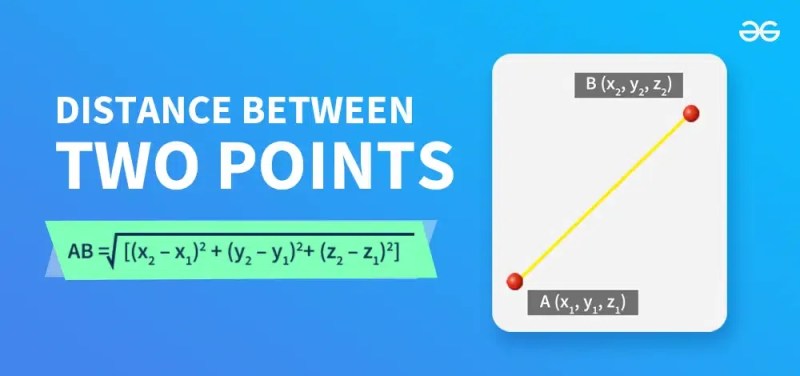
The formula for distance between two points operates on a fundamental geometric principle: the shortest distance between two points is a straight line. In a 2D plane, this translates to constructing a right triangle where the two legs are the horizontal and vertical differences between the points (\(\Delta x\) and \(\Delta y\)), and the hypotenuse is the distance \(d\). The formula squares these differences to eliminate negative values, sums them, and takes the square root to return to the original units of measurement.Extending this to three dimensions adds a \(z\)-coordinate, yielding:
\[ d = \sqrt{(x_2 - x_1)^2 + (y_2 - y_1)^2 + (z_2 - z_1)^2} \]
This expansion mirrors how higher-dimensional spaces (e.g., 4D spacetime in relativity) incorporate additional terms. The formula’s power lies in its scalability—whether you’re measuring the distance between two pixels on a screen or the separation between galaxies, the underlying logic remains identical.
Key Benefits and Crucial Impact
The formula for distance between two points is more than a mathematical curiosity; it’s a problem-solving engine. In physics, it defines the metric space of Euclidean geometry, enabling precise calculations of motion, force, and energy. Engineers use it to optimize structural designs, ensuring bridges and buildings withstand stress by minimizing material strain over distances. Even in biology, it helps model molecular interactions, where the distance between atoms determines chemical reactions.Its impact extends to technology, where algorithms for machine learning rely on distance metrics (e.g., Euclidean distance) to classify data, recommend products, or detect anomalies. The formula’s efficiency—requiring only basic arithmetic—makes it ideal for real-time applications, from autonomous vehicles adjusting trajectories to astronomers calculating interstellar distances. Without it, the digital world’s spatial intelligence would collapse.
"Mathematics is the music of reason," —James Joseph Sylvester.
The formula for distance between two points is its most universal melody, resonating across every field that demands precision in space.
Major Advantages
- Universality: Applies identically across 2D, 3D, and n-dimensional spaces, making it adaptable to any coordinate system.
- Computational Efficiency: Requires only subtraction, squaring, summation, and a square root—minimal operations for high-speed processing.
- Foundational for Algorithms: Powers clustering (k-means), nearest-neighbor searches, and neural network training in AI.
- Physical Accuracy: Directly models real-world distances in navigation, astronomy, and engineering simulations.
- Educational Accessibility: Introduces students to algebra, geometry, and calculus in an intuitive, hands-on manner.
Comparative Analysis
| Euclidean Distance (Standard Formula) | Alternative Distance Metrics |
|---|---|
| Calculates straight-line distance; assumes perfect spatial continuity. | Manhattan distance (taxicab geometry) accounts for grid-based paths (e.g., city blocks). |
| Optimal for unobstructed environments (e.g., open space, physics simulations). | Hamming distance measures binary data differences (e.g., DNA sequencing, error correction). |
| Sensitive to scale; larger coordinate differences amplify distance. | Cosine similarity focuses on angle between vectors, ignoring magnitude (used in text/NLP). |
| Extends naturally to higher dimensions without modification. | Mahalanobis distance incorporates covariance, useful in statistics for multivariate data. |
Future Trends and Innovations
As technology advances, the formula for distance between two points will evolve in tandem. In quantum computing, distance metrics may redefine how we measure separations in non-Euclidean spaces, where traditional geometry fails. Meanwhile, augmented reality (AR) and virtual reality (VR) will demand more nuanced distance calculations to render 3D environments with photorealistic precision. Machine learning’s reliance on distance-based algorithms (e.g., support vector machines) will push for faster, more efficient implementations, possibly leveraging neuromorphic hardware.The rise of big data also introduces challenges: as datasets grow to millions of dimensions, the computational cost of Euclidean distance calculations becomes prohibitive. Innovations like locality-sensitive hashing (LSH) are already emerging to approximate distances without full computation, hinting at a future where the formula’s simplicity is preserved even as its applications grow exponentially complex.
Conclusion
The formula for distance between two points is a testament to the enduring power of mathematical abstraction. From the clay tablets of ancient Mesopotamia to the silicon chips of modern supercomputers, it has remained a constant—adapting, expanding, and enabling breakthroughs across disciplines. Its elegance lies not just in its simplicity, but in its ability to connect disparate fields, from the macroscopic (galactic distances) to the microscopic (atomic bonds).As we stand on the brink of new scientific frontiers—quantum mechanics, AI-driven simulations, and interplanetary exploration—the formula’s role will only grow. It is more than a tool; it is a lens through which we measure, understand, and shape the universe. In an era where data is the new currency, mastering this fundamental concept isn’t just about solving equations—it’s about unlocking the spatial logic that governs reality itself.
Comprehensive FAQs
Q: Can the formula for distance between two points be used in non-Euclidean spaces?
A: The standard Euclidean distance formula assumes flat space. In non-Euclidean geometries (e.g., spherical or hyperbolic), alternative metrics like great-circle distance (for spheres) or hyperbolic distance replace it. These account for curvature, which is critical in general relativity and GPS corrections.
Q: How does the formula change for higher dimensions?
A: The formula extends by adding squared differences for each coordinate. For example, in 4D spacetime (used in relativity), it becomes \(d = \sqrt{(x_2 - x_1)^2 + (y_2 - y_1)^2 + (z_2 - z_1)^2 + (t_2 - t_1)^2}\), where \(t\) represents time. The principle remains identical: sum the squares of differences and take the square root.
Q: Why is the Euclidean distance formula preferred in machine learning?
A: Euclidean distance is intuitive and computationally efficient, making it ideal for tasks like k-nearest neighbors (KNN) and clustering. However, in high-dimensional spaces, it can suffer from the "curse of dimensionality," where distances between points become artificially inflated. Alternatives like cosine similarity or Manhattan distance are often used to mitigate this.
Q: What real-world applications rely on the distance formula beyond geometry?
A: Beyond geometry, the formula underpins:
- Physics: Calculating potential energy between charged particles.
- Computer Graphics: Rendering 3D models and lighting effects.
- Biology: Modeling protein folding via atomic distances.
- Economics: Measuring financial risk using distance-based correlations.
Q: Are there any limitations to using the Euclidean distance formula?
A: Yes. In obstructed environments (e.g., urban navigation), it may overestimate actual travel distance due to barriers. Additionally, in high-dimensional data, Euclidean distance can become less meaningful as all points appear equidistant—a phenomenon addressed by techniques like dimensionality reduction (PCA) or using alternative metrics.
Q: How is the distance formula implemented in programming?
A: In Python, you’d use:
import mathLibraries like NumPy generalize this for n-dimensional arrays:
def distance(x1, y1, x2, y2):
return math.sqrt((x2 - x1)2 + (y2 - y1)2)
from numpy.linalg import normFor large-scale applications, optimized C++ or GPU-accelerated implementations (e.g., CUDA) are often employed.
norm(np.array([x2 - x1, y2 - y1]))
Leave a Comment
Comments are moderated before appearing. The data you submit is processed according to the Privacy Policy of versiliasolutions.oneagency.co.