Decoding the One-Sample T-Test Formula: A Statistical Powerhouse Explained
Table of Contents
- The Complete Overview of the One-Sample T-Test Formula
- Historical Background and Evolution
- Core Mechanisms: How It Works
- Key Benefits and Crucial Impact
- Major Advantages
- Comparative Analysis
- Future Trends and Innovations
- Conclusion
- Comprehensive FAQs
- Q: When should I use the one-sample t-test formula instead of a z-test?
- Q: What happens if my data violates the normality assumption?
- Q: Can the one-sample t-test formula be used for categorical data?
- Q: How do degrees of freedom affect the t-test results?
- Q: What’s the difference between a one-tailed and two-tailed t-test?
The one-sample t-test formula is not just a mathematical tool; it is the linchpin of inferential statistics, allowing researchers to compare a single sample mean against a known population parameter. Whether validating a new drug’s efficacy against a standard benchmark or assessing whether a manufacturing process meets quality thresholds, this statistical method provides a rigorous framework for decision-making. Its elegance lies in its simplicity: by quantifying the discrepancy between observed data and an established norm, it transforms raw measurements into actionable insights.
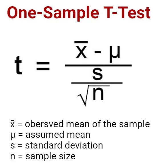
Yet, despite its ubiquity, the one-sample t-test formula is often misunderstood—confused with its two-sample counterpart or misapplied due to assumptions about normality and variance. The formula itself, \( t = \frac{\bar{X} - \mu_0}{s / \sqrt{n}} \), belies its depth. Here, \(\bar{X}\) represents the sample mean, \(\mu_0\) the hypothesized population mean, \(s\) the sample standard deviation, and \(n\) the sample size. The ratio of deviation from expectation to variability reveals whether the observed sample could plausibly arise from the assumed population—or if it signals a meaningful departure.
The power of this test lies in its ability to bridge theory and practice. From clinical trials to quality control, industries rely on the one-sample t-test formula to validate hypotheses with confidence. But its proper application demands more than memorization; it requires an understanding of when to use it, how to interpret its output, and the pitfalls of ignoring its underlying assumptions.

The Complete Overview of the One-Sample T-Test Formula
The one-sample t-test formula serves as a gateway to parametric hypothesis testing, offering a structured approach to evaluate whether a sample mean differs significantly from a known population mean. Unlike non-parametric alternatives, this method assumes the data follows a normal distribution—a critical consideration that dictates its applicability. The formula’s structure, \( t = \frac{\bar{X} - \mu_0}{s / \sqrt{n}} \), encapsulates the core logic: if the calculated \( t \)-value exceeds a critical threshold (determined by degrees of freedom and significance level), the null hypothesis—that the sample mean equals the population mean—is rejected.What sets the one-sample t-test apart is its reliance on the sample’s own variability (\( s \)) rather than a pre-determined population standard deviation. This adaptability makes it versatile, though it introduces sensitivity to sample size and distribution shape. Small samples, for instance, may require adjustments like Welch’s t-test if normality is questionable, while large samples often relax distributional assumptions via the Central Limit Theorem.
Historical Background and Evolution
The foundations of the one-sample t-test formula were laid in the early 20th century by William Sealy Gosset, who published his work under the pseudonym "Student" in 1908. Gosset’s contributions to small-sample statistics at Guinness Brewery addressed a practical problem: how to assess the quality of beer batches with limited data. His solution, the t-distribution, provided a robust alternative to the normal distribution when sample sizes were small, directly influencing the development of the one-sample t-test formula.Over the decades, the method evolved alongside advancements in computing and statistical theory. The advent of digital tools democratized its application, allowing researchers across disciplines to test hypotheses with unprecedented precision. Today, the one-sample t-test formula remains a staple in academic research, industrial quality assurance, and even social sciences, where it helps distinguish signal from noise in experimental results.
Core Mechanisms: How It Works
At its core, the one-sample t-test formula operates by standardizing the difference between the sample mean (\(\bar{X}\)) and a hypothesized population mean (\(\mu_0\)) using the sample’s standard error (\( s / \sqrt{n} \)). This standardization yields a \( t \)-statistic, which is then compared to a critical value from the t-distribution table or evaluated via p-value calculation. The degrees of freedom (\( n - 1 \)) adjust the distribution’s shape, accounting for sample variability.The test’s logic hinges on two competing hypotheses: the null hypothesis (\( H_0: \bar{X} = \mu_0 \)) and the alternative (\( H_1: \bar{X} \neq \mu_0 \), \( H_1: \bar{X} > \mu_0 \), or \( H_1: \bar{X} < \mu_0 \)). If the calculated \( t \)-value falls in the rejection region (beyond the critical \( t \)-value at a chosen significance level, e.g., 0.05), the null hypothesis is rejected, implying the sample mean is statistically different from \(\mu_0\). This binary outcome—reject or fail to reject—drives decision-making in fields where precision is non-negotiable.
Key Benefits and Crucial Impact
The one-sample t-test formula is a cornerstone of evidence-based research, offering a statistically rigorous method to validate hypotheses against a known standard. Its ability to quantify uncertainty through p-values and confidence intervals provides clarity in ambiguous scenarios, such as determining whether a new teaching method improves student performance compared to historical averages. This clarity is invaluable in domains where stakes are high, from pharmaceutical trials to policy evaluations.Beyond its practical utility, the one-sample t-test formula fosters reproducibility. By standardizing the testing process, it ensures that results are interpretable across studies, reducing variability in conclusions. This consistency is particularly critical in collaborative research, where multiple teams may analyze similar datasets under different conditions.
"Statistics is the grammar of science. The one-sample t-test formula is one of its most precise sentences—concise yet capable of conveying complex truths about data."
— Ronald Fisher, Statistician and Geneticist
Major Advantages
- Precision in Small Samples: Unlike z-tests, which require large samples, the one-sample t-test formula adjusts for small-sample variability using the t-distribution, making it reliable even with limited data.
- Flexibility in Hypothesis Testing: It accommodates one-tailed and two-tailed tests, allowing researchers to tailor the analysis to specific research questions (e.g., detecting improvements vs. any deviation).
- Interpretability: The \( t \)-statistic and p-value provide intuitive metrics for assessing significance, bridging the gap between raw data and actionable insights.
- Assumption Transparency: The method explicitly requires normality and independence, forcing researchers to validate these assumptions before proceeding—preventing misapplication.
- Widespread Software Support: Implementation in tools like R, Python (SciPy), and SPSS ensures accessibility, with automated calculations reducing human error.
Comparative Analysis
| One-Sample T-Test Formula | Two-Sample T-Test |
|---|---|
| Compares a single sample mean (\(\bar{X}\)) to a known population mean (\(\mu_0\)). | Compares means of two independent samples to determine if they differ. |
| Uses sample standard deviation (\( s \)) and degrees of freedom (\( n - 1 \)). | May use pooled variance (if equal variances assumed) or separate variances (Welch’s t-test). |
| Assumes normality of the sample distribution. | Assumes normality in each sample, though robust to violations with large \( n \). |
| Formula: \( t = \frac{\bar{X} - \mu_0}{s / \sqrt{n}} \). | Formula: \( t = \frac{\bar{X}_1 - \bar{X}_2}{\sqrt{\frac{s_1^2}{n_1} + \frac{s_2^2}{n_2}}} \). |
Future Trends and Innovations
As data volumes grow and computational power expands, the one-sample t-test formula is evolving to meet new challenges. Machine learning integration is enabling adaptive versions of the test, where prior knowledge or Bayesian frameworks refine hypothesis testing. Additionally, non-parametric alternatives (e.g., permutation tests) are gaining traction, offering robustness when normality assumptions falter.The future may also see hybrid approaches, combining the precision of the one-sample t-test formula with the flexibility of modern statistical learning. For instance, bootstrapping methods could supplement traditional t-tests, providing more accurate confidence intervals for complex datasets. These innovations will likely preserve the formula’s core logic while extending its applicability to big data and high-dimensional spaces.
Conclusion
The one-sample t-test formula remains a bedrock of statistical analysis, offering a time-tested method to evaluate hypotheses with clarity and rigor. Its ability to distill complex datasets into actionable \( t \)-values and p-values underscores its enduring relevance. However, its proper use hinges on understanding its assumptions, limitations, and the context in which it is applied.As research methodologies advance, the one-sample t-test formula will continue to adapt, but its fundamental principles—comparing observed data to a standard while accounting for variability—will endure. For practitioners, mastering this tool is not just about memorizing the formula but recognizing when and how to wield it effectively in an ever-expanding statistical landscape.
Comprehensive FAQs
Q: When should I use the one-sample t-test formula instead of a z-test?
A: Use the one-sample t-test formula when your sample size is small (typically \( n < 30 \)) or when the population standard deviation is unknown. The z-test assumes a known population standard deviation and relies on the normal distribution, making it suitable for large samples where the Central Limit Theorem ensures normality of the sampling distribution.
Q: What happens if my data violates the normality assumption?
A: If your data is not normally distributed, especially with small sample sizes, the one-sample t-test formula may yield unreliable results. Consider non-parametric alternatives like the Wilcoxon signed-rank test or bootstrap methods. For large samples, the Central Limit Theorem often mitigates this issue, but always check normality via Shapiro-Wilk tests or Q-Q plots.
Q: Can the one-sample t-test formula be used for categorical data?
A: No, the one-sample t-test formula is designed for continuous numerical data. For categorical outcomes, use chi-square tests or Fisher’s exact test. If your data is ordinal, consider non-parametric tests like the Mann-Whitney U test or Kruskal-Wallis test.
Q: How do degrees of freedom affect the t-test results?
A: Degrees of freedom (\( n - 1 \)) determine the shape of the t-distribution, which is heavier-tailed than the normal distribution for small samples. As degrees of freedom increase, the t-distribution converges to the normal distribution. This means critical \( t \)-values become less extreme, making it easier to reject the null hypothesis with larger samples.
Q: What’s the difference between a one-tailed and two-tailed t-test?
A: A one-tailed t-test is used when you have a directional hypothesis (e.g., "the sample mean is greater than \(\mu_0\)"), focusing all alpha (significance level) in one tail of the distribution. A two-tailed test is non-directional (e.g., "the sample mean differs from \(\mu_0\)"), splitting alpha between both tails. One-tailed tests are more powerful for detecting effects in a specific direction but risk false positives if misapplied.
Leave a Comment
Comments are moderated before appearing. The data you submit is processed according to the Privacy Policy of versiliasolutions.oneagency.co.