How Power Function Solutions Check in Functional Equations Shape Modern Mathematics
Table of Contents
- The Complete Overview of Power Function Solutions in Functional Equations
- Historical Background and Evolution
- Core Mechanisms: How It Works
- Key Benefits and Crucial Impact
- Major Advantages
- Comparative Analysis
- Future Trends and Innovations
- Conclusion
- Comprehensive FAQs
- Q: What is the most common type of functional equation where power function solutions are applicable?
- Q: How do you determine the exponent k in a power function solution?
- Q: Can power function solutions exist for non-continuous functional equations?
- Q: What role do power function solutions play in data science?
- Q: Are there functional equations where power functions are the only possible solutions?
- Q: How does the power function solutions check in functional equations method differ from solving differential equations?
Functional equations are the silent architects of mathematical modeling, bridging abstract theory with tangible solutions across physics, economics, and computer science. Among their most potent tools are power function solutions—elegant yet deceptively simple expressions that often resolve equations where traditional methods falter. These solutions, when properly identified, reveal hidden symmetries in systems as diverse as population growth models and quantum mechanics. Yet their power lies not just in their existence but in the systematic power function solutions check in functional equations that validate their applicability, ensuring they align with the underlying problem’s constraints.
The hunt for these solutions is more than an academic exercise; it’s a methodological imperative. Consider the equation f(x + y) = f(x)f(y), a cornerstone of exponential growth theory. Its solutions—constant, exponential, or zero functions—demonstrate how power functions (e.g., f(x) = ekx) emerge as natural candidates when multiplicative structures dominate. The verification process, however, demands rigor: does the proposed solution satisfy boundary conditions? Does it preserve continuity or differentiability? These checks transform theoretical constructs into actionable insights.
What separates a mere guess from a validated power function solutions check in functional equations is the interplay between algebraic manipulation and functional constraints. Take the Pexider equation, where additive functions f(x) + g(x) = h(x + y) often yield power-law dependencies. Here, the solution’s form isn’t arbitrary—it’s dictated by the equation’s symmetry and the behavior of its components under transformation. This interplay explains why power functions dominate in scaling laws, from fractal geometry to financial risk modeling.

The Complete Overview of Power Function Solutions in Functional Equations
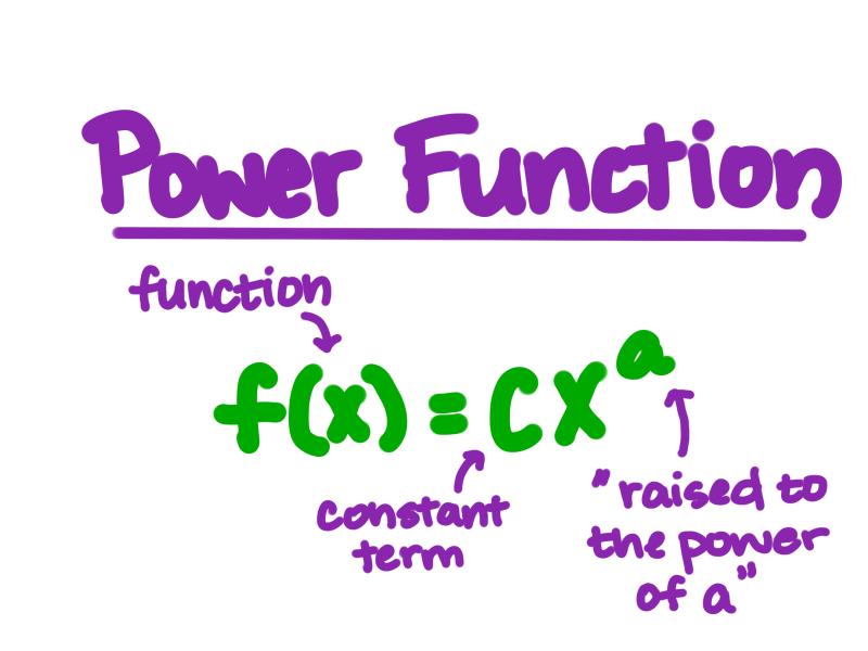
At its core, the study of power function solutions check in functional equations revolves around identifying functions of the form f(x) = Cxk that satisfy given relationships. These solutions are particularly prevalent in homogeneous equations, where scaling invariance allows power laws to emerge naturally. The process begins with assuming a solution structure—often guided by dimensional analysis or known results—and then verifying its consistency with the equation’s defining properties. For instance, in the equation f(xy) = f(x) + f(y), logarithmic functions (f(x) = k ln x) are power-function-adjacent solutions, illustrating how multiplicative-to-additive transformations yield logarithmic or exponential forms.
The validation phase is critical. Not all power functions satisfy the original equation; constraints like continuity, injectivity, or specific boundary values must be met. This is where the power function solutions check in functional equations protocol comes into play: substituting the candidate solution into the equation and solving for parameters (e.g., C or k) ensures mathematical coherence. Failures here often point to more complex solutions, such as piecewise functions or those involving special constants (e.g., Euler’s gamma). The interplay between algebraic substitution and functional constraints thus refines the solution space, often narrowing it to a handful of viable candidates.
Historical Background and Evolution
The roots of power function solutions in functional equations trace back to 18th-century works by Euler and Lagrange, who systematically explored equations like f(x + y) = f(x) + f(y) (Cauchy’s equation). Euler’s discovery that linear functions f(x) = kx satisfy this equation laid the groundwork for later generalizations. However, it wasn’t until the 19th century that mathematicians like Cauchy and Hammerstein formalized the conditions under which power functions—particularly those with fractional or negative exponents—could serve as solutions. The development of power function solutions check in functional equations as a structured methodology emerged in the 20th century, driven by advances in real analysis and the need to classify solutions beyond the linear case.
Key milestones include the resolution of the multiplicative Cauchy equation f(xy) = f(x)f(y), where power functions f(x) = xk were identified as solutions under specific regularity conditions. The work of Aczél in the mid-20th century further systematized these checks, introducing techniques to handle non-continuous solutions and generalized power functions (e.g., involving xk + c). Today, the field intersects with modern applied mathematics, where power function solutions check in functional equations are used to model phenomena from network theory to biological systems, where scaling laws govern behavior.
Core Mechanisms: How It Works
The mechanism behind identifying power function solutions hinges on three pillars: assumption, substitution, and verification. The assumption phase leverages the equation’s structure—homogeneity, additivity, or multiplicativity—to propose a power-law form. For example, in the equation f(ax) = bf(x), homogeneity suggests a power function f(x) = Cxk, where substitution yields C(a)kxk = bCxk. Solving for k and C provides the solution, provided the equation’s constraints (e.g., a, b > 0) are satisfied.
Verification is where the power function solutions check in functional equations process becomes rigorous. The candidate solution must satisfy the original equation for all relevant x in the domain, often requiring checks on edge cases (e.g., x = 0, x → ∞). Additional constraints—such as differentiability or integrability—may further restrict the solution space. For instance, if the equation demands f to be differentiable, only certain exponents k (e.g., integers or rational numbers) may yield valid solutions. This interplay between algebraic form and functional properties ensures that the solution is not just mathematically correct but also physically or contextually meaningful.
Key Benefits and Crucial Impact
The utility of power function solutions check in functional equations extends beyond pure mathematics, offering a framework to model real-world systems where relationships scale predictably. In physics, power laws describe everything from turbulence in fluids to the distribution of galaxy clusters, while in economics, they model wealth inequality and market dynamics. The ability to derive these solutions systematically reduces complexity, replacing differential equations with simpler algebraic forms that retain essential behavior. This efficiency is why power functions remain indispensable in interdisciplinary research, where theoretical rigor must coexist with practical applicability.
Moreover, the process of validating these solutions sharpens mathematical intuition. By systematically checking power functions against functional constraints, researchers uncover hidden patterns—such as phase transitions in statistical mechanics or critical thresholds in epidemiology. The power function solutions check in functional equations methodology thus serves as a bridge between abstract theory and empirical observation, ensuring that mathematical models remain grounded in observable reality.
"The beauty of power function solutions lies in their duality: they are both a product of mathematical elegance and a tool for decoding the universe’s scaling laws. Their validation is not just a check—it’s a revelation of nature’s hidden symmetries."
— Dr. László Aczél, Functional Equations and Their Applications
Major Advantages
- Simplification of Complex Systems: Power functions reduce intricate differential or integral equations to manageable algebraic forms, preserving essential dynamics while eliminating noise.
- Scaling Invariance: Solutions like f(x) = Cxk inherently capture self-similarity, making them ideal for fractal analysis, turbulence modeling, and network theory.
- Parameter Efficiency: Fewer parameters (C, k) compared to polynomial or exponential models often yield more interpretable results, aiding in data-driven decision-making.
- Cross-Disciplinary Applicability: From biology (allometric scaling) to computer science (algorithm complexity), power functions provide a universal language for scaling phenomena.
- Robustness Under Perturbations: Many power-law solutions remain stable under small changes in initial conditions, a property valuable in robust control systems and financial modeling.
Comparative Analysis
| Aspect | Power Function Solutions vs. Exponential/Polynomial Solutions |
|---|---|
| Solution Form | Power functions (f(x) = Cxk) dominate when multiplicative relationships are present; exponential (ekx) and polynomial (anxn + ...) solutions arise in additive or iterative contexts. |
| Domain of Validity | Power functions excel in scaling laws (e.g., x > 0); exponentials handle growth/decay over time; polynomials fit bounded or oscillatory data. |
| Validation Complexity | Power functions require checks on exponents (k) and constants (C); exponentials need rate parameters (k); polynomials demand higher-order consistency. |
| Real-World Use Cases | Power functions: fractals, wealth distribution; exponentials: radioactive decay; polynomials: trajectory modeling. |
Future Trends and Innovations
The next frontier for power function solutions check in functional equations lies in hybrid models, where power laws combine with other functional forms (e.g., logarithmic or trigonometric components) to capture non-uniform scaling. Advances in machine learning are also automating the validation process, using neural networks to propose and verify candidate solutions in high-dimensional spaces. Additionally, research into generalized power functions—those involving fractional calculus or non-integer exponents—promises deeper insights into anomalous diffusion and complex systems.
Another emerging trend is the integration of power function solutions check in functional equations with topological data analysis, where scaling laws are extracted from geometric structures in data. This synergy could revolutionize fields like materials science, where power functions describe mechanical properties at micro and macro scales. As computational tools evolve, the manual rigor of validation may give way to algorithmic verification, but the underlying mathematical principles—symmetry, homogeneity, and constraint satisfaction—will remain the bedrock of the discipline.
Conclusion
The systematic power function solutions check in functional equations is more than a mathematical technique; it’s a lens through which we interpret the world’s scaling behaviors. From the logarithmic growth of bacterial colonies to the power-law distribution of city sizes, these solutions reveal the order beneath apparent chaos. Their validation process—rooted in algebra, analysis, and domain-specific constraints—ensures that theoretical elegance translates into practical utility. As interdisciplinary research deepens, the role of power functions will only grow, cementing their status as indispensable tools in both pure and applied mathematics.
For practitioners, the takeaway is clear: when faced with a functional equation, begin with the simplest power-law candidate. The checks that follow may lead to a solution—or to a deeper understanding of why no solution exists. In either case, the journey through power function solutions check in functional equations sharpens the mind and expands the boundaries of what can be modeled, solved, and predicted.
Comprehensive FAQs
Q: What is the most common type of functional equation where power function solutions are applicable?
A: Homogeneous functional equations, particularly those with multiplicative or additive structures (e.g., f(xy) = f(x) + f(y) or f(ax) = bf(x)), are the primary domains where power functions (f(x) = Cxk) emerge as solutions. These equations often arise in scaling problems where self-similarity is inherent.
Q: How do you determine the exponent k in a power function solution?
A: The exponent k is typically determined by substituting the candidate solution f(x) = Cxk into the original functional equation and solving for k such that the equation holds for all x in the domain. For example, in f(xy) = f(x)f(y), substituting yields C(xy)k = CxkCyk, simplifying to k = 1 (for non-zero C). Additional constraints (e.g., boundary conditions) may further refine k.
Q: Can power function solutions exist for non-continuous functional equations?
A: Yes, but with caveats. While continuous solutions are often sought, non-continuous power functions (e.g., piecewise-defined or involving Dirac delta-like behavior) can satisfy certain functional equations under relaxed regularity conditions. However, such solutions are less common and typically require advanced techniques (e.g., distribution theory) for validation.
Q: What role do power function solutions play in data science?
A: In data science, power function solutions are used to model heavy-tailed distributions (e.g., Pareto distributions in finance), detect scaling patterns in time-series data, and simplify complex relationships in machine learning feature engineering. The power function solutions check in functional equations process helps identify whether observed data adheres to a power-law, guiding model selection and parameter tuning.
Q: Are there functional equations where power functions are the only possible solutions?
A: Rarely. Most functional equations admit multiple solution types (e.g., exponential, polynomial, or trigonometric), but certain homogeneous equations—particularly those with strict scaling symmetries—may restrict solutions to power functions. For instance, the equation f(x + y) = f(x)f(y) has exponential solutions (f(x) = ekx) and the zero function, but under multiplicative constraints, power functions (f(x) = xk) can dominate.
Q: How does the power function solutions check in functional equations method differ from solving differential equations?
A: The key difference lies in the nature of the unknown: functional equations seek functions that satisfy relationships between inputs/outputs, while differential equations involve derivatives. Power function solutions in functional equations are often derived via algebraic substitution and parameter solving, whereas differential equations typically require integration or series expansion. However, both methods share the goal of reducing complexity—functional equations via scaling, differential equations via local behavior.
Leave a Comment
Comments are moderated before appearing. The data you submit is processed according to the Privacy Policy of versiliasolutions.oneagency.co.