How Big O Notation Deciphers Algorithm Efficiency
Table of Contents
- The Complete Overview of Big O Notation
- Historical Background and Evolution
- Core Mechanisms: How It Works
- Key Benefits and Crucial Impact
- Major Advantages
- Comparative Analysis
- Future Trends and Innovations
- Conclusion
- Comprehensive FAQs
- Q: Why do we ignore constants and lower-order terms in big O notation?
- Q: Can big O notation describe space complexity?
- Q: What’s the difference between best-case, average-case, and worst-case big O?
- Q: How does big O relate to NP-completeness? A: NP-complete problems require O(2ⁿ) or worse solutions for exact solutions. Big O helps classify these problems, showing why brute-force methods are impractical for large inputs (e.g., the Traveling Salesman Problem). Q: Is big O notation only for computer science?
- Q: What’s a common misconception about big O?
- Q: How do I analyze an algorithm’s big O if it has nested loops?
- Q: Can big O notation be used for approximate algorithms?
Big O notation isn’t just a mathematical curiosity—it’s the silent architect behind every scalable application, from Google’s search engine to the blockchain networks powering cryptocurrency. When developers debate whether a sorting algorithm runs in O(n log n) versus O(n²), they’re not just splitting hairs; they’re deciding between a system that handles millions of queries per second and one that grinds to a halt under moderate load. The notation itself, with its asymptotic shorthand, strips away implementation details to reveal the fundamental truth about how an algorithm behaves as input size grows. This isn’t theoretical pedantry; it’s the difference between a product that thrives and one that fails under pressure.
Yet for all its ubiquity, big O notation remains misunderstood. Many engineers treat it as a checkbox—something to mention in interviews or whiteboard sessions—without grasping its deeper implications. The notation’s elegance lies in its simplicity: a single symbol (O(n), O(1), O(2ⁿ)) can encapsulate the scalability of an entire system. But simplicity often masks complexity. Behind those symbols are decades of mathematical rigor, trade-offs between time and space, and the unspoken rules that govern when an algorithm is truly "efficient." To master it is to gain a superpower: the ability to predict performance before writing a single line of code.
The notation’s origins trace back to 19th-century number theory, but its modern form was crystallized in the 1960s by Donald Knuth, who recognized its utility in computer science. Before big O, engineers relied on vague terms like "fast" or "slow," leading to costly surprises when systems scaled. Knuth’s work formalized the idea of asymptotic analysis—focusing not on exact runtime but on how growth rates compare as inputs become arbitrarily large. This shift was revolutionary. Suddenly, developers could reason about algorithms in terms of orders of magnitude, making it possible to compare a quadratic algorithm (O(n²)) to a logarithmic one (O(log n)) without running benchmarks. The notation didn’t just describe performance; it predicted it.

The Complete Overview of Big O Notation
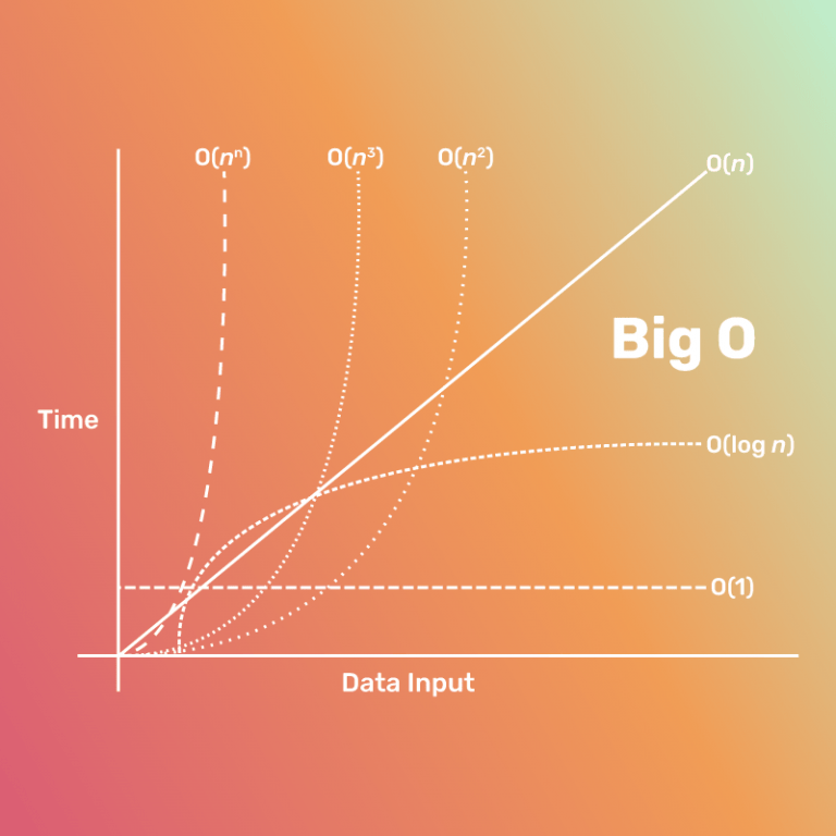
Big O notation is the lens through which computer scientists examine algorithmic efficiency, distilling complex runtime behaviors into a few symbolic expressions. At its core, it answers a single question: How does the time or space required by an algorithm grow as the input size increases? The notation ignores constants and lower-order terms, focusing instead on the dominant factor that dictates scalability. For example, an algorithm with a runtime of 3n² + 2n + 10 is classified as O(n²) because, for large n, the n² term dwarfs the others. This abstraction allows engineers to compare algorithms without getting bogged down in hardware-specific details or implementation quirks.The power of big O lies in its generality. Whether analyzing a hash table’s O(1) average-case lookup or a brute-force search’s O(2ⁿ) exponential complexity, the notation provides a universal language. It’s not about precise measurements but about relative performance. A O(log n) algorithm will always outperform a O(n) one as n approaches infinity, regardless of the constant factors. This makes it indispensable in fields ranging from database optimization to machine learning, where data sizes can span orders of magnitude. Yet, the notation’s simplicity can be misleading—misapplying it (e.g., conflating best-case, average-case, and worst-case scenarios) can lead to catastrophic misjudgments in system design.
Historical Background and Evolution
The seeds of big O notation were sown in 1894 by Paul Bachmann, who used similar asymptotic ideas to analyze number-theoretic functions. However, it was Edmund Landau who formalized the notation in his 1909 work, Handbuch der Lehre von der Verteilung der Primzahlen, using O() to describe bounds on error terms in number theory. The notation’s leap into computer science came decades later, as early programmers grappled with the limitations of punch-card machines and mainframes. The 1960s and 1970s saw its adoption in algorithm analysis, thanks in large part to Knuth’s The Art of Computer Programming, where he redefined it for computational contexts.Knuth’s contributions were pivotal. He introduced the Theta (Θ) notation to describe tight bounds and the Omega (Ω) notation for lower bounds, creating a family of tools to dissect algorithmic behavior. His work demystified complexity, showing that big O wasn’t just about runtime but also about space complexity—how much memory an algorithm consumes as input grows. The notation’s adoption accelerated with the rise of structured programming and the need for predictable performance in real-time systems. Today, it’s a cornerstone of computer science education, taught alongside basic data structures in introductory courses. Its evolution reflects a broader shift: from ad-hoc programming to engineering systems that can scale reliably.
Core Mechanisms: How It Works
Big O notation operates on two fundamental principles: asymptotic analysis and growth rate comparison. Asymptotic analysis ignores fixed costs (like setup time) and focuses on how an algorithm’s resource usage scales with input size. For instance, an algorithm that processes n elements with a fixed overhead of 1000 operations is still O(n) because the linear term dominates as n grows. Growth rate comparison, meanwhile, pits algorithms against each other. A O(n log n) sorting algorithm (like Merge Sort) will always outperform a O(n²) one (like Bubble Sort) for sufficiently large datasets, even if the constants favor the latter in small-scale tests.The notation’s formal definition is rooted in mathematical limits. An algorithm f(n) is O(g(n)) if there exist constants c > 0 and n₀ such that f(n) ≤ c·g(n) for all n ≥ n₀. This means the function f(n) is bounded above by g(n) up to a constant factor, beyond some point. For example, 2n + 5 is O(n) because for n ≥ 5, 2n + 5 ≤ 4n. The notation’s strength lies in its ability to abstract away implementation details, allowing engineers to focus on the essential behavior of an algorithm. However, this abstraction can also be a pitfall—real-world performance often depends on constants and lower-order terms that big O deliberately obscures.
Key Benefits and Crucial Impact
Big O notation is more than a theoretical tool; it’s a practical necessity for building systems that can handle growth. In an era where datasets can swell from kilobytes to petabytes overnight, the difference between a O(n) and a O(n log n) algorithm isn’t just academic—it’s existential. Consider a social media platform processing billions of user interactions. A poorly chosen algorithm could turn a real-time feature into a latency nightmare, driving users to competitors. The notation forces engineers to confront trade-offs: Should you prioritize faster lookups (O(1)) at the cost of higher memory usage? Or accept slower queries (O(log n)) for a more compact data structure?The notation’s impact extends beyond performance. It shapes architectural decisions, influencing everything from database indexing strategies to the choice between recursive and iterative implementations. In distributed systems, big O analysis helps determine whether a task can be parallelized effectively. Even in hardware design, the notation informs cache optimization and pipeline efficiency. Without it, scaling would be a guessing game—relying on trial and error rather than principled reasoning. As one computer scientist once noted:
"Big O notation is the compass that guides us through the fog of implementation details, pointing toward the horizon of scalability." — Donald Knuth (paraphrased)
Major Advantages
- Scalability Prediction: Big O reveals how an algorithm behaves as input size grows, allowing engineers to anticipate bottlenecks before they materialize.
- Algorithm Comparison: It provides a standardized way to evaluate trade-offs between time and space complexity, e.g., O(n) time vs. O(n log n) space.
- Language Agnostic: The notation transcends programming languages, making it a universal tool for analyzing pseudocode, assembly, or high-level implementations.
- Design Clarity: By focusing on asymptotic behavior, it helps teams prioritize optimizations that yield the most significant long-term benefits.
- Theoretical Foundation: It bridges computer science and mathematics, enabling rigorous analysis of problems like NP-completeness and polynomial-time reductions.
Comparative Analysis
| Complexity Class | Characteristics and Examples |
|---|---|
| Constant Time (O(1)) | Fixed runtime regardless of input size. Examples: Array indexing, hash table lookups (average case). Ideal for high-frequency operations. |
| Logarithmic Time (O(log n)) | Runtime grows logarithmically with input size. Examples: Binary search, divide-and-conquer algorithms. Efficient for sorted data. |
| Linear Time (O(n)) | Runtime scales directly with input size. Examples: Simple loops, linear search. Balanced for moderate-sized datasets. |
| Quadratic Time (O(n²)) | Runtime grows with the square of input size. Examples: Bubble Sort, nested loops. Impractical for large n but simple to implement. |
Future Trends and Innovations
As data sizes continue to explode and hardware diversifies (from quantum processors to edge devices), big O notation will evolve to address new challenges. One emerging trend is the analysis of amortized complexity, where algorithms like dynamic arrays (O(1) average-case insertion) hide their occasional O(n) operations behind a smoother asymptotic profile. Another frontier is parallel complexity, where the notation must account for distributed systems where O(n) on a single core becomes O(n/p) across p processors. Additionally, the rise of machine learning has sparked interest in statistical complexity, where algorithms’ performance is analyzed in terms of data distribution rather than raw input size.The notation may also adapt to approximate computing, where exact results are sacrificed for speed in applications like real-time analytics. As quantum algorithms mature, big O may need to incorporate quantum complexity classes (e.g., BQP), which defy classical asymptotic analysis. Ultimately, the notation’s enduring relevance lies in its ability to adapt—remaining a lens through which engineers can navigate an increasingly complex computational landscape.
Conclusion
Big O notation is not just a tool; it’s a mindset. It teaches engineers to think in terms of growth, trade-offs, and fundamental limits—lessons that apply far beyond algorithm design. Whether optimizing a search engine or architecting a blockchain, the notation provides the framework to ask the right questions: What happens when the dataset doubles? When it grows a thousandfold? The answers shape the systems we build, determining which ideas succeed and which fail under pressure.Yet, the notation’s true value lies in its humility. It doesn’t promise exact predictions or eliminate the need for benchmarking, but it does offer a language to discuss efficiency without ambiguity. In an industry obsessed with "scaling," big O is the compass that keeps us grounded in reality. Ignore it at your peril; master it, and you master the art of building systems that last.
Comprehensive FAQs
Q: Why do we ignore constants and lower-order terms in big O notation?
A: Constants and lower-order terms become negligible as input size grows. For example, in 2n + 100, the 100 is dwarfed by 2n when n is large. Big O focuses on the dominant term because it dictates long-term scalability.
Q: Can big O notation describe space complexity?
A: Yes. Space complexity uses the same notation to describe how memory usage scales with input size. For example, a recursive Fibonacci algorithm may have O(n) space complexity due to the call stack.
Q: What’s the difference between best-case, average-case, and worst-case big O?
A: Best-case (Ω) describes the fastest possible runtime (e.g., O(1) for a sorted array in linear search). Average-case (Θ) accounts for typical inputs, while worst-case (O) guarantees performance under all conditions. Hash tables are O(1) average-case but O(n) worst-case if collisions dominate.
Q: How does big O relate to NP-completeness?
A: NP-complete problems require O(2ⁿ) or worse solutions for exact solutions. Big O helps classify these problems, showing why brute-force methods are impractical for large inputs (e.g., the Traveling Salesman Problem).
Q: Is big O notation only for computer science?
A: No. It’s used in operations research, economics (e.g., analyzing algorithmic trading strategies), and even biology (e.g., modeling protein folding complexity). Its principles apply anywhere growth rates matter.
Q: What’s a common misconception about big O?
A: Many assume O(n²) is "always bad," but context matters. For small n, a quadratic algorithm may outperform a O(n log n) one due to lower constants. The notation is about asymptotic behavior, not absolute performance.
Q: How do I analyze an algorithm’s big O if it has nested loops?
A: Multiply the complexities of nested structures. For example, two nested O(n) loops result in O(n²). If the inner loop runs m times where m ≤ n, the complexity is O(n²). If m is constant, it’s O(n).
Q: Can big O notation be used for approximate algorithms?
A: Yes, but with caveats. Approximate algorithms (e.g., in machine learning) may trade accuracy for speed, leading to complexities like O(n log n) with a probabilistic guarantee (e.g., "99% accurate in O(n) time").
Leave a Comment
Comments are moderated before appearing. The data you submit is processed according to the Privacy Policy of versiliasolutions.oneagency.co.