How to Find Interquartile Range: The Definitive Statistical Guide for Precision Analysis
Table of Contents
- The Complete Overview of How to Find Interquartile Range
- Historical Background and Evolution
- Core Mechanisms: How It Works
- Key Benefits and Crucial Impact
- Major Advantages
- Comparative Analysis
- Future Trends and Innovations
- Conclusion
- Comprehensive FAQs
- Q: What is the difference between interquartile range and range?
- Q: Can I use IQR for normally distributed data?
- Q: How do I calculate IQR in Excel?
- Q: Why is IQR important in box plots?
- Q: What are Tukey’s fences, and how do they relate to IQR?
- Q: Can IQR be negative?
- Q: How does sample size affect IQR?
- Q: Is IQR used in hypothesis testing?
The interquartile range (IQR) is the statistical measure that separates the middle 50% of a dataset from its extremes. Unlike standard deviation, which can be skewed by outliers, IQR provides a robust way to understand data dispersion—critical for fields like finance, healthcare, and quality control. Many professionals overlook its simplicity, assuming it requires advanced tools. In reality, how to find interquartile range is a foundational skill that can be applied with basic arithmetic or spreadsheet functions, yet its implications for data integrity are profound.
The IQR isn’t just a theoretical concept; it’s a practical tool used to identify anomalies, assess risk, and design experiments. For instance, a biostatistician might use it to determine whether a patient’s lab results fall within an expected range, while a supply chain analyst could apply it to predict inventory fluctuations. The method’s elegance lies in its resistance to outliers—a flaw many other statistical measures share. Yet, despite its utility, miscalculations are common, often due to confusion over quartile definitions or dataset ordering.
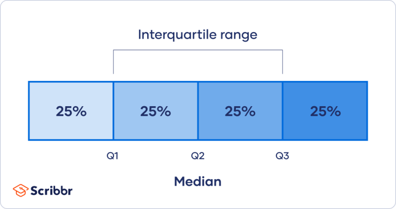
Understanding how to calculate the interquartile range begins with recognizing that it’s not a single value but a range derived from two quartiles: Q1 (the 25th percentile) and Q3 (the 75th percentile). The difference between these two points (Q3 – Q1) reveals the spread of the central data, excluding the top and bottom 25%. This approach is particularly valuable in skewed distributions, where mean and median may mislead. Whether you’re analyzing survey responses, financial returns, or manufacturing defects, IQR offers clarity where other metrics falter.

The Complete Overview of How to Find Interquartile Range
The interquartile range (IQR) is a measure of statistical dispersion that quantifies the spread of the middle 50% of a dataset. Unlike the range (which is simply the difference between the maximum and minimum values), IQR focuses on the interquartile spread, making it less sensitive to extreme values. This property is why it’s favored in robust statistical analysis, particularly in fields where outliers can distort results—such as quality assurance, economics, and environmental science.To find the interquartile range, you first identify the first quartile (Q1) and the third quartile (Q3). Q1 is the median of the first half of the data, while Q3 is the median of the second half. The IQR is then calculated as Q3 minus Q1. This method ensures that only the central data points influence the measure, providing a more accurate representation of variability in skewed or asymmetrical distributions. For example, in a dataset of household incomes, the IQR would reveal the typical income range of the middle class without being skewed by billionaire outliers.
Historical Background and Evolution
The concept of quartiles and the interquartile range traces back to early 19th-century statistics, when researchers sought ways to summarize large datasets without relying solely on mean and standard deviation. The British statistician Karl Pearson and French mathematician Francis Edgeworth later formalized percentile-based measures, but it was the work of American statistician George W. Snedecor in the 1930s that popularized quartiles as a tool for descriptive statistics. Snedecor’s emphasis on robustness—particularly in agricultural and industrial data—laid the groundwork for IQR’s adoption in modern analytics.Today, how to find interquartile range is taught as a cornerstone of exploratory data analysis (EDA), alongside measures like variance and standard deviation. Its evolution reflects a shift toward more resilient statistical methods, especially as datasets grew larger and more complex. In the 1970s, the rise of computing allowed for automated quartile calculations, democratizing the technique. Now, tools like Python’s `numpy.percentile` or Excel’s `QUARTILE.INC` function make it accessible to non-specialists, though understanding the underlying mechanics remains essential for accurate interpretation.
Core Mechanisms: How It Works
The process of calculating the interquartile range begins with ordering the dataset from smallest to largest. Once sorted, the median (Q2) divides the data into two halves. Q1 is then the median of the lower half, and Q3 is the median of the upper half. For an even number of observations, the median may be averaged from two central points, while for odd counts, the middle value is excluded when splitting the data. The IQR is simply the difference between Q3 and Q1, representing the range within which the central 50% of data resides.For instance, consider a dataset of exam scores: [60, 65, 70, 75, 80, 85, 90, 95]. The median (Q2) is 77.5, splitting the data into [60, 65, 70, 75] and [80, 85, 90, 95]. Q1 is the median of the first half (67.5), and Q3 is the median of the second half (87.5). The IQR is 87.5 – 67.5 = 20. This method ensures that only the central data points influence the result, making it far less susceptible to outliers than the range. Software tools automate this process, but manual calculation reinforces understanding of the dataset’s structure.
Key Benefits and Crucial Impact
The interquartile range is more than a statistical curiosity—it’s a practical tool for identifying data trends, detecting anomalies, and making informed decisions. Unlike standard deviation, which can be inflated by extreme values, IQR provides a stable measure of spread, making it ideal for real-world applications where outliers are common. Industries from healthcare to manufacturing rely on it to assess variability in processes, ensuring consistency and quality.In finance, for example, analysts use IQR to evaluate the volatility of asset returns without being derailed by market crashes or speculative bubbles. Similarly, in quality control, manufacturers monitor IQR to detect deviations in production lines before defects escalate. The measure’s robustness extends to social sciences, where survey data often contains skewed responses. By focusing on the central 50%, researchers avoid misinterpretations that could arise from relying on mean or median alone.
"The interquartile range is the compass of statistical analysis—it points you toward the heart of your data, where the most reliable insights reside." — Dr. John Tukey, Pioneer of Exploratory Data Analysis
Major Advantages
- Robustness to Outliers: Unlike range or standard deviation, IQR is unaffected by extreme values, making it ideal for skewed distributions.
- Clear Data Interpretation: Provides a straightforward measure of central spread, aiding in visualizations like box plots.
- Widely Applicable: Used in finance, healthcare, engineering, and social sciences for risk assessment and quality control.
- Simplicity in Calculation: Requires only basic arithmetic once quartiles are identified, accessible even without advanced tools.
- Foundation for Advanced Analysis: Serves as a prerequisite for techniques like Tukey’s fences for outlier detection.
Comparative Analysis
| Interquartile Range (IQR) | Standard Deviation |
|---|---|
| Measures spread of the middle 50% of data; resistant to outliers. | Measures average deviation from the mean; sensitive to extreme values. |
| Calculated as Q3 – Q1; requires quartile identification. | Calculated as the square root of variance; requires all data points. |
| Preferred for skewed distributions or small datasets. | Preferred for normally distributed data with few outliers. |
| Used in box plots, Tukey’s fences, and robust statistical methods. | Used in hypothesis testing, regression analysis, and confidence intervals. |
Future Trends and Innovations
As datasets grow in size and complexity, the demand for robust statistical measures like IQR will continue to rise. Machine learning models, which often rely on feature scaling, increasingly incorporate quartile-based normalization to handle skewed data. Additionally, advancements in computational tools are making it easier to calculate IQR dynamically, even in real-time analytics. Future innovations may integrate IQR with big data platforms, enabling automated outlier detection in streaming datasets.The integration of how to find interquartile range into predictive analytics is another emerging trend. By combining IQR with machine learning algorithms, analysts can improve model accuracy by focusing on data distributions rather than raw values. For instance, financial institutions might use IQR to refine risk models, while healthcare providers could leverage it to identify patient outliers in clinical trials. As statistics evolve, the IQR’s role as a cornerstone of data integrity will only strengthen.
Conclusion
Mastering how to find interquartile range is essential for anyone working with data, from students analyzing survey results to professionals in data-driven industries. Its ability to filter out noise and highlight central trends makes it indispensable in fields where precision matters. While tools like Excel or Python can automate calculations, understanding the underlying mechanics ensures accurate interpretation and application.The IQR’s enduring relevance lies in its simplicity and effectiveness. Whether you’re a researcher, analyst, or decision-maker, this measure provides clarity in the face of variability. By incorporating it into your statistical toolkit, you gain a reliable method to assess data spread—one that stands the test of outliers and complexity.
Comprehensive FAQs
Q: What is the difference between interquartile range and range?
A: The range is the difference between the maximum and minimum values in a dataset, making it highly sensitive to outliers. The interquartile range (IQR), however, focuses on the spread of the middle 50% of data (Q3 – Q1), providing a more robust measure of variability.
Q: Can I use IQR for normally distributed data?
A: While IQR is useful for any distribution, it’s particularly valuable for skewed or asymmetric data. For normally distributed datasets, standard deviation is often preferred, but IQR can still be used for outlier detection (e.g., Tukey’s fences).
Q: How do I calculate IQR in Excel?
A: In Excel, use the `QUARTILE.INC` function to find Q1 and Q3. For example:
Q1 = QUARTILE.INC(range, 1)
Q3 = QUARTILE.INC(range, 3)
Then subtract Q1 from Q3 to get the IQR.
Q: Why is IQR important in box plots?
A: Box plots visually represent the IQR as the height of the box, showing the interquartile spread. The "whiskers" extend to 1.5×IQR beyond Q1 and Q3, helping identify outliers. This makes IQR a key component of exploratory data visualization.
Q: What are Tukey’s fences, and how do they relate to IQR?
A: Tukey’s fences define outliers as values below Q1 – 1.5×IQR or above Q3 + 1.5×IQR. This method uses IQR to detect anomalies without assuming a normal distribution, making it robust for real-world data.
Q: Can IQR be negative?
A: No, the interquartile range is always non-negative because it’s calculated as Q3 – Q1, where Q3 ≥ Q1 by definition. A negative result would indicate an error in quartile calculation.
Q: How does sample size affect IQR?
A: For small datasets (n < 20), quartiles may be less stable, leading to larger IQR fluctuations. Larger samples provide more reliable quartile estimates, making IQR a consistent measure of spread.
Q: Is IQR used in hypothesis testing?
A: While IQR isn’t directly used in traditional hypothesis tests (like t-tests), it’s valuable for non-parametric methods and robustness checks. For example, it helps assess whether assumptions of normality hold before applying parametric tests.
Leave a Comment
Comments are moderated before appearing. The data you submit is processed according to the Privacy Policy of versiliasolutions.oneagency.co.