How to Find the Interquartile Range: The Definitive Statistical Tool for Data Analysis
Table of Contents
- The Complete Overview of How to Find the Interquartile Range
- Historical Background and Evolution
- Core Mechanisms: How It Works
- Key Benefits and Crucial Impact
- Major Advantages
- Comparative Analysis
- Future Trends and Innovations
- Conclusion
- Comprehensive FAQs
- Q: What is the difference between the interquartile range and standard deviation?
- Q: Can the interquartile range be negative?
- Q: How do I calculate the interquartile range in Excel?
- Q: Why is the interquartile range important in box plots?
- Q: What happens if my dataset has an even number of observations when calculating quartiles?
- Q: Can the interquartile range be used for hypothesis testing?
- Q: Is the interquartile range affected by the sample size?
The interquartile range (IQR) is the statistical measure that separates the middle 50% of a dataset from its extremes. Unlike standard deviation, which can be skewed by outliers, the IQR provides a robust way to assess data spread—critical for fields like finance, healthcare, and quality control. Yet, despite its importance, many professionals overlook how to find the interquartile range accurately, leading to misinterpreted insights or flawed decision-making.
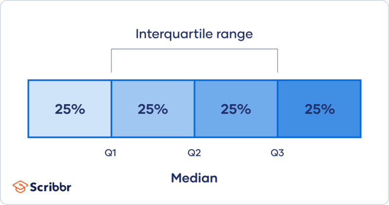
At its core, how to find the interquartile range hinges on identifying the first (Q1) and third (Q3) quartiles, then subtracting Q1 from Q3. This simple operation reveals the range where the central data resides, offering clarity in datasets with skewed distributions or outliers. Mastering this technique isn’t just about memorizing formulas; it’s about understanding how quartiles divide data and why the IQR outperforms alternatives like range or variance in certain contexts.
The IQR’s power lies in its simplicity and resilience. While tools like Excel or Python can automate the process, grasping the manual method ensures deeper analytical rigor. Whether you’re analyzing stock market volatility, patient response times in clinical trials, or manufacturing defect rates, knowing how to calculate the interquartile range empowers you to filter noise and focus on meaningful patterns.

The Complete Overview of How to Find the Interquartile Range
The interquartile range is a cornerstone of descriptive statistics, offering a clear snapshot of data variability without distortion from extreme values. To determine the interquartile range, you first partition the ordered dataset into four equal segments using quartiles. The lower quartile (Q1) marks the 25th percentile, while the upper quartile (Q3) represents the 75th percentile. The difference between Q3 and Q1 (IQR = Q3 − Q1) quantifies the spread of the central data, making it indispensable for box plots, outlier detection, and comparative analyses.The process of finding the interquartile range varies slightly depending on whether your dataset contains an odd or even number of observations. For even-sized datasets, quartiles are calculated by interpolating values between ranked data points, whereas odd-sized datasets use median-based partitioning. This distinction ensures precision, especially in small samples where rounding errors can skew results. Tools like statistical software or graphing calculators streamline these calculations, but manual computation remains essential for validating automated outputs and understanding underlying principles.
Historical Background and Evolution
The concept of quartiles emerged in the late 19th century as statisticians sought ways to summarize data distributions more effectively than simple measures like mean or range. Early statisticians, including Francis Galton and Karl Pearson, recognized that dividing data into quartiles could mitigate the influence of outliers, a problem plaguing traditional measures of dispersion. The interquartile range, as a derivative of quartiles, gained prominence in the 20th century with the rise of robust statistics—particularly in fields where data integrity was paramount, such as quality control and social sciences.Today, how to find the interquartile range is taught alongside foundational statistical methods, reflecting its enduring relevance. The IQR’s ability to complement other metrics (e.g., median for central tendency) has cemented its role in exploratory data analysis. Historical advancements in computational tools have further democratized its use, allowing practitioners across disciplines to apply it without deep mathematical expertise. Yet, the core methodology remains unchanged: quartiles as dividers, IQR as the measure of central spread.
Core Mechanisms: How It Works
The interquartile range is calculated by first ordering the dataset from smallest to largest. For a dataset with n observations, the position of Q1 and Q3 is determined using the formula:Position = (p/100) × (n + 1), where p is the percentile (25 for Q1, 75 for Q3). If the position is not an integer, interpolation between adjacent values is required. For example, in a dataset of 10 values, Q1 would be at position (0.25 × 11) = 2.75, meaning the value is 75% between the 2nd and 3rd ordered observations.
This method ensures that the IQR captures the spread of the middle 50% of data, excluding the top and bottom 25%. Unlike the range (max − min), which is sensitive to outliers, the IQR provides a stable measure of variability. For instance, in a skewed distribution, the IQR might reveal that most values cluster tightly around the median, while the range exaggerates the influence of a few extreme points. This precision is why how to calculate the interquartile range is prioritized in robust statistical analyses.
Key Benefits and Crucial Impact
The interquartile range is more than a calculation—it’s a lens through which data’s true variability becomes visible. By focusing on the central 50% of observations, it reduces the impact of outliers, which can distort other measures like standard deviation. This makes the IQR particularly valuable in fields such as finance, where a single extreme market event could mislead analysts relying on traditional dispersion metrics. Similarly, in healthcare, the IQR helps clinicians assess patient response times without overemphasizing anomalous cases.Understanding how to find the interquartile range also enhances interpretability in visual tools like box plots. The IQR defines the "box" in a box-and-whisker plot, while whiskers extend to 1.5 × IQR to flag outliers. This visual representation distills complex datasets into actionable insights, from identifying process inefficiencies in manufacturing to spotting trends in consumer behavior. The IQR’s versatility extends to hypothesis testing, where it informs non-parametric methods resistant to non-normal distributions.
"The interquartile range is the statistician’s shield against the tyranny of outliers—it reveals the heart of the data where other measures falter." — John Tukey, Statistician and Data Visualization Pioneer
Major Advantages
- Robustness to Outliers: Unlike standard deviation, the IQR remains unaffected by extreme values, providing a reliable measure of central dispersion.
- Simplicity and Interpretability: The calculation involves basic arithmetic (Q3 − Q1), making it accessible even to non-statisticians.
- Foundation for Box Plots: The IQR defines the central box in box plots, enabling clear visualization of data spread and outliers.
- Non-Parametric Flexibility: Works effectively with skewed or non-normal distributions, where parametric methods (e.g., t-tests) may fail.
- Decision-Making Clarity: Helps identify data clusters, anomalies, and trends without the noise of extreme values.
Comparative Analysis
| Metric | Interquartile Range (IQR) |
|---|---|
| Definition | Range of the middle 50% of data (Q3 − Q1). |
| Sensitivity to Outliers | Low (ignores top/bottom 25%). |
| Use Case | Robust dispersion, box plots, non-normal data. |
| Calculation Complexity | Moderate (requires quartile determination). |
Future Trends and Innovations
As data science evolves, the interquartile range is being integrated into advanced analytical frameworks. Machine learning models now use IQR-based feature scaling to normalize datasets before training, reducing the impact of skewed variables. In big data contexts, algorithms automatically compute quartiles for massive datasets, enabling real-time IQR analysis in streaming environments. Future innovations may also see IQR applied in explainable AI, where transparency in data distribution is critical for model interpretability.The rise of automated statistical tools (e.g., Python’s `pandas`, R’s `dplyr`) has made how to find the interquartile range more accessible, but the underlying principles remain unchanged. As industries generate larger, messier datasets, the IQR’s robustness will continue to distinguish it from less resilient metrics. Emerging fields like genomics and climate science are likely to adopt IQR-based methods for handling noisy, high-dimensional data, ensuring its relevance for decades to come.
Conclusion
Mastering how to calculate the interquartile range is a gateway to more accurate data interpretation. Whether you’re a data analyst refining predictive models or a researcher validating experimental results, the IQR provides a stable foundation for understanding variability. Its simplicity belies its power, offering a clear alternative to metrics vulnerable to outliers or skewed distributions.For practitioners, the key takeaway is balance: while tools can automate IQR calculations, a manual understanding ensures trust in the results. As data grows in complexity, the IQR’s role as a robust measure of central spread will only expand, cementing its place alongside median and mean as a statistical essential.
Comprehensive FAQs
Q: What is the difference between the interquartile range and standard deviation?
A: The interquartile range (IQR) measures the spread of the middle 50% of data and is robust to outliers, while standard deviation quantifies overall dispersion, including extreme values. IQR is preferred for skewed data or when outliers are present.
Q: Can the interquartile range be negative?
A: No. Since Q3 is always greater than or equal to Q1 in ordered datasets, the IQR (Q3 − Q1) is always non-negative. A negative result would indicate data processing errors.
Q: How do I calculate the interquartile range in Excel?
A: Use the `QUARTILE.INC` function to find Q1 and Q3 (e.g., `=QUARTILE.INC(range, 1)` for Q1), then subtract Q1 from Q3. Alternatively, `PERCENTILE.INC(range, 0.25)` and `PERCENTILE.INC(range, 0.75)` can be used.
Q: Why is the interquartile range important in box plots?
A: The IQR defines the "box" in a box plot, representing the central 50% of data. Whiskers extend to 1.5 × IQR, helping visualize outliers and data distribution at a glance.
Q: What happens if my dataset has an even number of observations when calculating quartiles?
A: For even n, quartiles are calculated by interpolating between ranked values. For example, Q1 at position 2.75 in a 10-value dataset is 75% between the 2nd and 3rd values: `value = (0.75 × (value3 − value2)) + value2`.
Q: Can the interquartile range be used for hypothesis testing?
A: Yes. The IQR informs non-parametric tests like the Mann-Whitney U test or Kruskal-Wallis test, where normality assumptions are relaxed. It also helps define confidence intervals for medians.
Q: Is the interquartile range affected by the sample size?
A: The IQR’s calculation method adjusts for sample size (e.g., `(p/100) × (n + 1)`), but its robustness to outliers remains consistent across small and large datasets. Larger samples may yield more precise quartile estimates.
Leave a Comment
Comments are moderated before appearing. The data you submit is processed according to the Privacy Policy of versiliasolutions.oneagency.co.